
Morpheus v2 Release Notes
Check out the new goodies in Morpheus v2
We are very proud to announce a new major release for our multicellular modeling environment:
🎉 Morpheus v2 🎉
Many many things have changed since the first official release in 2014. We released new modeling features such as MembraneProperties, new plugins such as a new Protrusion plugin, implemented a very generic Logger plugin, properly scaled the neighborhoods in CPM simulations, included new data visualization tools such as TiffPlotter, improved SBML support and enabled external bash and python script. We reworked our MorpheusML model definition language to be more generic, while remaining backward compatible and improved the automatic conversion of old models into Morpheus v2 format (FixBoard). We refactored the symbol tracking to create the computational graph, and introduced the concept of spatial scoping. We improved the appearance and stability of the GUI in multiple ways including a new in-app documentation browser which now support $\LaTeX$ equations. And, not unimportantly, we have open-sourced our code and welcomed a number of external contributors to the development team!
In fact, there are way too many new things to list here. To be fair, many of the new features have been released in intermediate versions and have been available in version 1.9.2 (which was silently released earlier this year) and have since then been tested in the wild. Nevertheless, Morpheus v2 is the first official and stable release and we have saved some nice goodies for this official new release.
In this post, we will take a look at the most significant changes from the perspective of a modeller. The goal here is not to be comprehensive, but to introduce a number of useful features you may not know about.
Table of Contents
General
Open Source
Already two years ago now, we have open sourced Morpheus under a permissive BSD license. All our code is hosted at our GitLab repo allowing everyone to fork, clone, or pull and to submit issues. We’re also moving our user and developer documentation to the wiki. Currently, we are moving from our old Morpheus homepage to these GitLab pages – the ones you are reading now.
These steps are aimed to create and expand Morpheus as a community-driven open source project. We therefore highly appreciate our current external contributors and welcome new developers to help make Morpheus better and more useful.
Extensible Framework
Morpheus now has a plugin architecture to allow external developers to add their own functionality, e.g. CellType plugins adding modeling new cellular behaviors and new Analysis plugins with custom-made data analysis tools.
Great care has been taken to facilitate the integration of new plugins into the framework such that newly developer plugins appear in the GUI with proper options and defaults, they can be coupled to other plugins and that they are automatically scheduled.
This new plugin architecture allows developers to create their own custom plugins that are hopefully contributed back to the community for all to use. We have already received a number of plugins from external contributors and we are looking forward to your merge requests.
Funding
We have secured funding for the further development, maintenance of Morpheus from the following sources:
- BMBF e:Med Systems Medicine network
- DFG Research Software Sustainability programme (e-Research Technologies)
- BMBF Computational Life Sciences programme
Modeling
Expressions Everywhere
You can now use mathematical symbolic expressions everywhere. Instead of assigning a value, you can write an expression, giving a great flexibility in writing more generic models and coupling different sub-models.
For example, you can flexibly initialize your simulation. Instead of specifying a lattice position explicitly like so "200,100,0", you can now say "size.x/2, size.y/2, 0" to put something in the middle of your 2D lattice (where Lattice/Size/symbol="size"). This will ensure that the position is still in the middle if you change the lattice size later on.
Or, you can reduce the temperature of your cellular Potts model over time to model simulated annealing (assuming TimeSymbol="time"):
<MetropolisKinetics temperature="max(0, 10 - time/250)">

Expressions will come in handy in many unexpected places. In fact, it is hard to overestimate the flexibility that the use of math expressions provides in your modeling work.
Membrane Properties
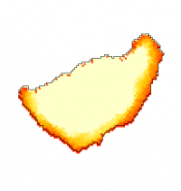
Cells are not isotropic and many exhibit polarity, an asymmetric distributions of proteins along their membrane. To represent anisotropy of cellular properties in Morpheus, we have introduced the concept of MembraneProperty.
A MembraneProperty is a scalar field mapped to cell membrane in polar coordinates using a circular (2D) or spherical (3D) approximation of cell shape. They allow modeling of anisotropic cell behavior, e.g. unequal concentration of adhesive molecules, and even reaction-diffusion on membranes, e.g. to dynamically induce polarity.
For example, the cells in the simulation below are more adhesive along the east-west poles (yellow) than along the north-south poles (blue/black) which results in convergent extension of the tissue.
A MembraneProperty can also be used in membrane-bound reaction-diffusion processes to model e.g. cell polarization. In the example below, we have two cells that polarize after cell-cell contact. This is implemented using two diffusive MembraneProperties that are coupled according to the wave-pinning model of cell polarity. The cells adhere to each other with their polar domains, because we also made adhesion a function of the polarized MembraneProperty resulting in anisotropic adhesion.
Vector Fields
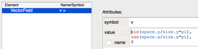
In addition to the standard scalar Field, Morpheus now also provides a VectorField construct. This allows you to define (x,y,z) vector data in a spatial field.
For example, here we define a VectorField v and initialize it:
… and simulate CPM cells that move along the vector field using DirectedMotion:
DirectedMotion.
Even better, we can update the vector field according to the movement of cells moving over it, modeling the extracelluar matrix, and have cells moving along the vector field, as a model of stigmergy:
Examples/CPM/Stigmergy_Vectorfield.xml).
Multiple Populations per CellType
To create complex initial conditions, Morpheus now supports the specification of multiple Populations of the same CellType in CellPopulations.
External Analysis
We often use external scripts to analyse the simulation results. Instead of doing such analysis post-hoc, the new Analysis plugin External allows you to run your scripts during simulation as part of your Morpheus job. This is very useful to run your e.g. python analysis pipeline automatically during or after simulation, and is crucial when doing automated parameter inference.
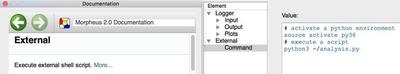
bash or python scripts during simulation as part of the Morpheus job.
Checkpointing
Morpheus now support checkpointing of the entire simulation state, including Fields, MembraneProperties and VectorFields. These can be used to restore a simulation state and rerun the simulation from this point onwards.
New CellType Plugins
ChangeCellType allows a cell to change its cell type of a cell based on a Condition.
AddCell can be used to add CPM cells during simulation based on a Condition and a location specified by a probability density function.
Protrusion is an actin-inspired feedback model that control shape and motility of CPM cells, as proposed by Niculescu et al., 2015.
Protrusion plugin models positive feedback of active membrane regions, inspired by actin dynamics.
Analysis Plugins
The Logger has been completely refactored and now provides a versatile interface to export simulation data and create beautiful visualizations.
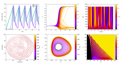
Logger plugin provides a versatile interface for data export and data visualization.
ContactLogger records the all aspects of cell-cell contacts, such as the cell ids of both cells and the length of the contact interface.
time	cell.id	cell.type	neighbor.id	neighbor.type	length
1640	1	0	2	0	15.2
1640	2	0	1	0	15.2
1660	1	0	2	0	17.6
1660	2	0	1	0	17.6
...
DependencyGraph allows you to specify the appearance of the symbol graph, as shown below
Other Changes
- The generalized
Mappernow takes care to map information between spatial contexts, replaces theCellReporter - The
Functionplugin now supports parametric functions and function overloading. - The value of a
Constantcan be provided via expression - Removed any remains of units in
timeandspace
GUI
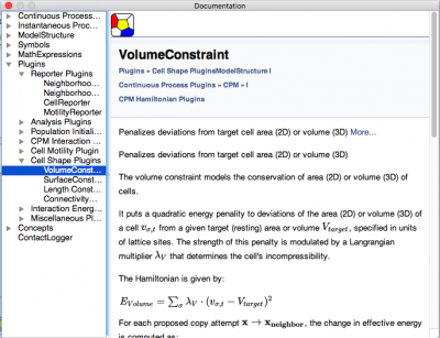
In-app Documentation
We improved the context-sensitive documentation by using doxygen-generated HTML rendering of the documentation (using QtWebKit). Docs are both context-sensitive and can be searched (using QtHelp framework) and can include $\LaTeX$-based maths (displayed using MathJax):
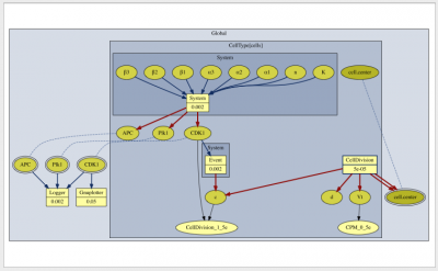
Symbol Graph
Morpheus automagically executes the simulation, based on tracking the dependencies of each symbol. Now, this symbol dependency graph is visualized and displayed in the GUI under the Description section.
This graph can be very useful to inspect the structure of your model and to trace information flows. The appearance of the graph can be configured in the new Analysis plugin DependencyGraph.
Create Movies
We have integrated a way to create mp4 movies from image sequences based on ffmpeg. This allows you to easily create a movie from images generated by Logger or Gnuplotter. This feature requires either ffmpeg (or avconv) to be installed on your system. If Morpheus cannot find it, please specify the excutable under Settings/Local.
Note: when used in a parameter sweep, it will generate movies for all simulations within the sweep.
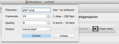
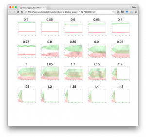
Image Table
To generate a visual overview of the results of a ParamSweep, we now provide a way to make a table of images or movies. The table is generated in HTML5 and will be opened in a web browser.
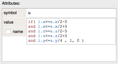
Multiline Attribute Editor
When using expressions as attributes, the single line editors were often too small. Now, Morpheus has multiline editor panel for expressions in attributes, when needed.
Parameter Sweeps
We have added an option to preset random seed for parameter sweeps, such that sweeps with stochastic (sub)models such as CPM are reproducible.
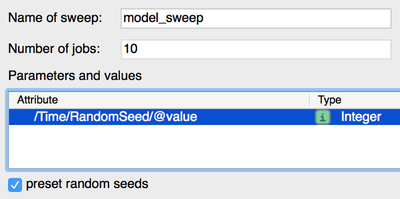
preset random seeds ensure stochastic parameter sweeps are reproducible.
We have also introduced a more parser-friendly format to replace the old sweep_summary.txt. Now, the information is separated into a header and a data file, structured like this:
sweep_header.csv:
Date	Tue Oct 16 2018
Time	13:59:01
Jobs	6
Params	2
P1	MorpheusModel/CellTypes/CellType[name=cells]/System/Constant[symbol=n]/@value
P2	MorpheusModel/CellTypes/CellType[name=cells]/System/Constant[symbol=K]/@value
sweep_data.csv
Folder	P1	P2
Example-CellCycle_sweep_82/Example-CellCycle_8481	3	0.2
Example-CellCycle_sweep_82/Example-CellCycle_8482	3	0.5
Example-CellCycle_sweep_82/Example-CellCycle_8483	4	0.2
Example-CellCycle_sweep_82/Example-CellCycle_8484	4	0.5
...
This makes it easier to post-process sweep data in external tools, e.g. using pandas.read_csv("sweep_data.csv", sep="\t").
SBML Support
SBML models can now be imported as ODE models in Global or in CellType. The first more closely reflects the original SBML model, and simulates the ODE as global variables. However, since the goal is often to extend the SBML model into a multicellular model, it is often more convenient to import the SBML model immediately as an intracellular ODE model. This can be achieved using the Into new CellType option.
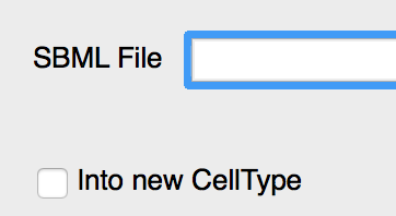
Global by default but can optionally be put in a new CellType.
Moreover, SBML import has been improved by the use of parametric function and covering a subset of MathML elements. Additionally, several issues converning SBML libraries under Mac and Windows have been resolved.
Drag’n’Drop External XML
You can now copy/paste or even drag/drop XML model snippets from external editors into Morpheus.
Simulation
Performance
Edge Tracking
Morpheus always used edge tracking to optimize performance. Instead of evaluating updates for all lattice sites, Morpheus only evaluates updates where things can actually change, namely along the cell edges. This makes CPM simulation much faster, but requires dynamically tracking the edges. We now optimized the memory layout of the tracked edges using periodic defragmentation such that looking up the relevant lattice sites is even faster.
Diffusion in Domains
Although diffusion in regular lattices was always parallelized, this was not the case when using Domains. Now, after implemeting a parallelization scheme for this special case, even diffusion in irregular Domains benefit from multithreading.
VTK Output
The VTKPlotter now supports writing binary files which induces a substantial performance boost for large 3D simulations.
Constant Expressions
A potential performance drawback of having “expression everywhere” is that they have to be evaluated at runtime. Even though Morpheus uses the lighting-fast muparser, evaluating expressions does have a performance impact. Therefore, Morpheus now detects expressions that are constant at initialisation time (by tracking whether they depend only on constant symbols) and precalculates the constant expressions only once.
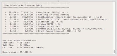
Profiling
To gain more insight in the performance of your simulation model, Morpheus now provides detailed information on execution time (wall time, CPU time) as well as peak memory usage. At the end of each simulation, a table is printed with an overview of the execution times (wall time) are listed per plugin.
Other Changes
- Fixes to initializers.
- Scheduling fixes to
DelayProperties. - Boundary conditions of
Fields can now be expressions.
MorpheusML
Scope and Spatial Scope
We introduced scoping in MorpheusML, analogous to lexical scoping in most programming languages. A symbol (or “name binding”) defined in a certain scope is invalid outside of this scope, but available in all sub-scoped, i.e. nested sections. This is analogous to the local variable scoping in most programming languages.
In MorpheusML, the top-most scope is Global. The other model sections that define their own scopes are CellType, System (including Trigger environments in some plugins) and Function. These scope are visualized in different shades of color in the symbol graph.
Symbols are inherited from the parental to the local scopes, but may be overwritten, even to differ in constness and granularity (e.g. Global/Constant may be overwritten by a System/Variable). The type of the symbol (scalar / vector), however, has to be conserved. In this way, global symbols can be used as default values.
As a special case, the CellType scope also represents a spatial compartment. In order to adhere to intuitive modelling logic, we apply spatial scoping. This implies that symbols defined in the CellType scope can override global symbols, but only in the spatial region its cells currently occupy. When a symbol is declared in all CellTypes, it automatically also becomes available in the global scope.
In the following example, a=1 is declared in the Global scope, and b=2 is declared in the System scope. The global variable result will yield 3.
<Global>
    <Constant symbol="a" value="1"/>
    <Variable symbol="result" value="0"/>

    <System solver="euler" time-step="1.0">
        <Constant symbol="b" value="2"/>
        <Rule symbol-ref="result">
            <Expression>a+b</Expression>
        </Rule>
    </System>
</Global>
Here, the global constant a=1 is overwritten in by the local constant a=2, such that result will yield 4.
<Global>
    <Constant symbol="a" value="1"/>
    <Variable symbol="result" value="0"/>

    <System solver="euler" time-step="1.0">
        <Constant symbol="a" value="2"/>
        <Constant symbol="b" value="2"/>
        <Rule symbol-ref="result">
            <Expression>a+b</Expression>
        </Rule>
    </System>
</Global>
Symbols can be re-used with different local scopes. Here, the symbol p is used in different CellTypes. In ct1, p is a Constant with value 0. In ct2, p is a Constant with value 1.0. In ct3, p denote a cell-bound Property and in ct4 it represents a MembraneProperty. And, because ‘p’ is defined in all CellTypes, it is automatically also available in the Global scope.
<CellTypes>
    <CellType class="biological" name="ct1">
        <Constant symbol="p" value="0"/>
    </CellType>
    <CellType class="biological" name="ct2">
        <Constant symbol="p" value="1.0"/>
    </CellType>
    <CellType class="biological" name="ct3">
        <Property symbol="p" value="1"/>
    </CellType>
    <CellType class="biological" name="ct4">
        <MembraneProperty symbol="p" value="l.x / size.x">
            <Diffusion rate="0.0"/>
        </MembraneProperty>
    </CellType>
</CellTypes>