Scaled Diffusion Coefficient to Obtain Identical Results in Physical Units Independent of Lattice Discretization
Persistent Identifier
Use this permanent link to cite or share this Morpheus model:
This example model demonstrates how to obtain consistent results in physical units together with the freedom to choose arbitrary lattice and time discretizations.
Introduction
Often, one starts to build a model with a particular lattice size and time scaling. Then later, one may want to run finer resolved simulations and has to increase the number of lattice nodes. However, that rather increases the spatial extensions and one needs to also rescale other parameters. This example model demonstrates how to do this right and strictly separate the physical scales from lattice and time discretizations.
Description
A PDE model is here defined in continuum space of size L.physical and discretized on the 1D interval [0,L.numerical], yielding a lattice spacing h = L.physical/L.numerical. The spatial location in physical units is then available for expressions, reporting and plotting as x.physical = x.numerical.x*h.
Likewise, the physical time interval [0,StopTime.physical] shall be discretized on the numerical interval [0,StopTime.numerical] with resulting physical time steps of duration tau = StopTime.physical/StopTime.numerical. The physical time is then available for expressions, reporting and plotting as time.physical = time.numerical*tau.
To analyse dynamic patterning due to reactions and diffusion, we added an activator-inhibitor model with fields a and i. The rate constants and diffusion constants shall be given in physical units and then the fluxes in the differential equations inside Global/System are scaled with tau.
The two diffusion coefficients D_a.physical and D_i.physical are given in physical units and then scaled inside Global/Field/Diffusion by the factor tau/(h*h) in response to the chosen discretizations.
Results
Simulations show the emergence of a Turing pattern from the initial condition for the field a = x.physical/L.physical. The profile of the activator variable is plotted as function of x.physical (Fig. 1) and time.physical (Fig. 2). As expected, these results are independent of the chosen numerical discretizations.
Here, we compare two runs with L.numerical = 80 on the left vs. L.numerical = 800 on the right. Apart from small numerical errors resulting from the relatively coarse discretization in the first case, the patterns are the same in space and time.
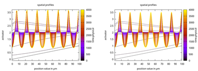
L.numerical = 80 on left and L.numerical = 800 on the right with the line color indicating time.
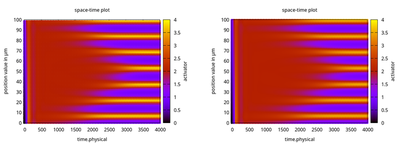
L.numerical = 80 on left and L.numerical = 800 on right with the color indicating activator values.
Model
Example_Scaled_Diffusion.xml
XML Preview
<?xml version='1.0' encoding='UTF-8'?>
<MorpheusModel version="4">
    <Description>
        <Details>Model ID:	https://identifiers.org/morpheus/M7992
  Software:	Morpheus (open source). Download from: https://morpheus.gitlab.io
Full title:	Scaled Diffusion Coefficient to Obtain Identical Results in Physical Units Independent of Lattice Discretization
Author:	R. Müller
Submitter:	L. Brusch
Curators:	R. Müller, J. Starruß, D. Jahn
Date:	03.01.2024
Comment:	Simulation of Turing pattern with the numerical diffusion coefficient scaled to the chosen spatial and temporal discretizations. Results are plotted over x.physical and time.physical and turn out independent of the numerical discretizations, as expected.
</Details>
        <Title>Example Scaled Diffusion</Title>
    </Description>
    <Space>
        <Lattice class="linear">
            <Neighborhood>
                <Order>optimal</Order>
            </Neighborhood>
            <Size symbol="size" value="L.numerical, 0, 0"/>
            <BoundaryConditions>
                <Condition type="noflux" boundary="-x"/>
                <Condition type="noflux" boundary="x"/>
            </BoundaryConditions>
        </Lattice>
        <SpaceSymbol symbol="x.numerical"/>
    </Space>
    <Time>
        <StartTime value="0"/>
        <StopTime symbol="StopTime.numerical" value="1"/>
        <TimeSymbol symbol="time.numerical"/>
    </Time>
    <Analysis>
        <ModelGraph format="dot" reduced="false" include-tags="#untagged"/>
        <Logger time-step="0.01">
            <Input force-node-granularity="false"/>
            <Output>
                <TextOutput/>
            </Output>
            <Plots>
                <Plot title="spatial profiles" time-step="-1">
                    <Style style="lines"/>
                    <Terminal terminal="png"/>
                    <X-axis>
                        <Symbol symbol-ref="x.physical"/>
                    </X-axis>
                    <Y-axis minimum="-0.1" maximum="3.7">
                        <Symbol symbol-ref="a"/>
                        <!--    <Disabled>
        <Symbol symbol-ref="i"/>
    </Disabled>
-->
                    </Y-axis>
                    <Color-bar>
                        <Symbol symbol-ref="time.physical"/>
                    </Color-bar>
                </Plot>
                <Plot title="space-time plot" time-step="-1">
                    <Style style="points"/>
                    <Terminal terminal="png"/>
                    <X-axis>
                        <Symbol symbol-ref="time.physical"/>
                    </X-axis>
                    <Y-axis>
                        <Symbol symbol-ref="x.physical"/>
                    </Y-axis>
                    <Color-bar>
                        <Symbol symbol-ref="a"/>
                    </Color-bar>
                </Plot>
            </Plots>
        </Logger>
    </Analysis>
    <Global>
        <Constant symbol="StopTime.physical" name="total time duration in seconds" value="4000"/>
        <Constant symbol="tau" name="time unit in seconds" value="StopTime.physical/StopTime.numerical"/>
        <Function symbol="time.physical">
            <Expression>time.numerical*tau</Expression>
        </Function>
        <Constant symbol="L.physical" name="system size in µm" value="100"/>
        <Constant symbol="L.numerical" value="80"/>
        <Constant symbol="h" name="lattice node length in µm" value="L.physical/L.numerical"/>
        <Function symbol="x.physical" name="position value in µm">
            <Expression>x.numerical.x*h</Expression>
        </Function>
        <Constant symbol="D_a.physical" name="diffusion constant of activator in µm²/sec" value="0.02"/>
        <Constant symbol="D_i.physical" name="diffusion constant of inhibitor in µm²/sec" value="1.0"/>
        <Field symbol="a" name="activator" value="x.physical/L.physical">
            <Diffusion rate="D_a.physical*tau/(h*h)"/>
        </Field>
        <Field symbol="i" name="inhibitor" value="0.1">
            <Diffusion rate="D_i.physical*tau/(h*h)"/>
        </Field>
        <System name="Activator-Inhibitor-Model" solver="Dormand-Prince [adaptive, O(5)]">
            <DiffEqn symbol-ref="a">
                <Expression>tau* ((rho*a^2) / i - mu_a * a + rho_a)</Expression>
            </DiffEqn>
            <DiffEqn symbol-ref="i">
                <Expression>tau* ((rho*a^2) - mu_i * i)</Expression>
            </DiffEqn>
            <Constant symbol="rho_a" name="" value="0.01"/>
            <Constant symbol="mu_i" value="0.03"/>
            <Constant symbol="mu_a" value="0.02"/>
            <Constant symbol="rho" value="0.001"/>
        </System>
    </Global>
</MorpheusModel>

Downloads
Files associated with this model: