Self-Organization of Leaf Polarity
Persistent Identifier
Use this permanent link to cite or share this Morpheus model:
A diffusible small-RNA-based Turing system dynamically coordinates organ polarity.
Introduction
The formation of a flat and thin leaf presents a developmentally challenging problem, requiring intricate regulation of top-bottom (adaxial-abaxial) polarity. The patterning principles controlling the spatial arrangement of these domains during organ growth have remained unclear. Scacchi et al. has shown that this regulation is achieved by an organ-autonomous Turing reaction-diffusion system centered on mobile small RNAs. They validated experimentally how a Turing dynamics transiently instructed by pre-patterned information is sufficient to self-sustain properly oriented polarity in a dynamic, growing organ.
Description
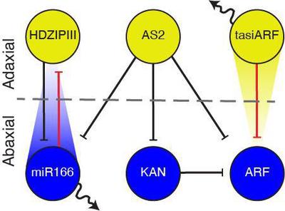
miR166 and tasiARF (mobile small RNAs) regulate top-bottom polarity on plants by limiting expression of their respective Class III HOMEODOMAIN LEUCINE ZIPPER (HD-ZIPIII) and AUXIN RESPONSE FACTOR3/4 (ARF3/4) targets, which, in conjunction with ASYMMETRIC LEAVES1/2 (AS) and KANADI (KAN) transcription factors, distinguish top versus bottom cell fate via further antagonistic interactions (Fig. 1).
The organizing principle underlying the GRN configuration that allows for the emergence and regulation of the top-bottom polarity, however, remains elusive. Scacchi et al. adopted a theoretical approach that considers all possible regulatory interactions, except those for miR166 and tasiARF, which only repress their specific targets. With the understanding that top and bottom cell fates are mutually exclusive, they addressed the possibility that a Turing reaction-diffusion system governs their domain organization. By using a high-throughput theoretical approach, Scacchi et al. identified a single 3-component network, the Leaf Polarity Model (LPM), as the minimal topological Turing model potentially capable to self-organize organ polarity. In this model, top determinants represented by distinct $\text{HDZIPIII}$ and $\text{AStasiARF}$ nodes form a negative feedback loop, and act in mutual opposition to bottom determinants, combined into a single $\text{miRKANARF}$ node (Fig. 2, Equation 1). Experimental validation has substantiated the architecture delineated by the LPM.
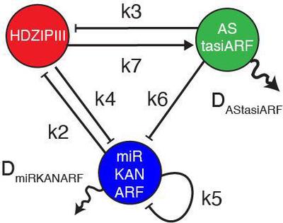
$$\left\{ \begin{aligned} \frac{\partial \text{HDZIPIII}}{\partial t} &= -0.5 \cdot \text{miRKANARF} + \text{AStasiARF} - \text{HDZIPIII}^3\\ \frac{\partial \text{miRKANARF}}{\partial t} &= -0.5 \cdot \text{HDZIPIII} - \text{miRKANARF} \pm \text{AStasiARF}\\ &\quad\ + D_{\text{miRKANARF}} \cdot \nabla^2 \cdot \text{miRKANARF}\\ \frac{\partial \text{AStasiARF}}{\partial t} &= \text{HDZIPIII}\\ &\quad\ + D_{\text{AStasiARF}} \cdot \nabla^2 \cdot \text{AStasiARF} \end{aligned} \right. $$
Results
1 – The LPM self-organizes a linearly-separated bipolar pattern in a 2-dimensional static grid of cells.
To address whether the LPM can coordinate the collective behaviour of cells to generate a spatial pattern at the organ level that resembles the bipolarity of a planar leaf, Scacchi et al. implemented a lattice of $30 \times 6$ hexagonal continuous static cells as a template to mimic the newly emerging leaf. To simulate inter- and intra-cellular chemical reactions at the organ level, they adopted a cellular agent-based model (ABM), where each cell elaborates the LPM and the diffusion and perception of mobile determinants occurs between contiguous cells relative to the cell-to-cell contact surface. They applied no-flux boundary conditions to both the top and bottom edges of the model template. Numerical simulations using Equation 1, $D_{\text{miRKANARF}} = 7.5 $, $D_{\text{AStasiARF}} = 75$, and initial random perturbations in a range of $\pm 0.1$ for $\text{miRKANARF}$ from the homogeneous steady-state $(\text{HDZIPIII}_0, \text{miRKANARF}_0, \text{AStasiARF}_0) = (0, 0, 0)$. The simulations generate a spatially stable pattern with $\text{HDZIPIII}$ and $\text{AStasiARF}$ out of phase from $\text{miRKANARF}$, but the pattern is variegated rather than bipolar (Fig. 3A, Supplementary_Code_1.xml).
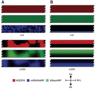
Supplementary_Code_1.xml). (B) In contrast, introducing $\text{miRKANARF}$ in the bottom cell layer as the initial condition, the system self-organizes over time into a bipolar pattern reminiscent of the adaxial-abaxial domain organization in a planar leaf (Supplementary_Code_2.xml). Simulation time $t = 300$. M-L, medio-lateral axis.
Considering that the adaxial-abaxial polarity network in young primordia from existing polarity, they next ran a numerical simulation as above, but with $\text{miRKANARF}$ in the bottom cell layer as the initial condition from the homogeneous steady-state as:
$$ \begin{aligned} \text{if} \left[\text{cell center on the}\ y\ \text{axis} \right] < \frac{\left[\text{size of}\ y\right]}{7}\ \text{then}\ \text{miRKANARF}_0 &= 5,\\\\ \text{otherwise}\ \text{miKANARF}_0 &= 0 \end{aligned} $$(Fig. 3B, Supplementary_Code_2.xml). Importantly, this ‘pre-patterned information’ is just an initial perturbation from the steady-state, and is not fixed over time, but instead immediately dissolves into the LPM during simulation. With the additional input of a polarly-localized rather than a stochastic initial perturbation, the simulation produces a bipolar pattern with $\text{HDZIPIII}$ and $\text{AStasiARF}$ marking the upper and $\text{miRKANARF}$ the lower cell layers. Therefore, in a defined cellular-based model, the LPM coordinates the collective behaviour of cells to self-organize into a linearly-separated bipolar tissue pattern, provided it perceives an initial polarized input for one of the system components. This transient pre-patterned information, in addition to generating bipolar stripes, also orients the stripes, such that polarity network components accumulate in the appropriate cell layers.
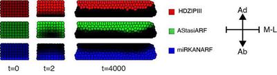
2 – The LPM self-organizes a robust linear polarity boundary in a growing cellular model
To assess whether the LPM can self-organize a robust bipolar pattern also in a growing template, Scacchi et al. generated a Cellular Potts model (CPM), in which cells are depicted as discrete and geometrically extended objects, and the plasma membrane and cell wall are simplified as a single entity (Supplementary_Code_3_main.xml). While this animal-based model can yield sliding effects between cells, this potential limitation was minimized by optimizing model conditions to mimic the immobility of plant cells. Moreover the focus is on the collective cell behaviour at the organ level, occasional subtle deviations at the scale of individual cells can be tolerated. The CPM through the Morpheus platform thus struck an ideal balance between rapid, high-throughput simulations and relevant representation of the biological system.
To reproduce the anisotropic growth of a developing leaf primordium in silico, Scacchi et al. implemented a constrained environment in which only anticlinal cell divisions occur as random events over time. Upon division, the content of each mother cell is equally distributed between the 2 daughter cells with a random perturbation of $\pm 0.001$. In addition, by setting a fixed target cell size, the daughter cells will expand to reach the mother cell size. In this way, cell division-driven growth is sufficient to generate a flat domain.
Following the proportions of a primordium shortly after emergence, they implemented the initial conditions as a population of $10 \times 6$ cells with no-flux boundary conditions for the upper and lower edges and an initial perturbation from the homogeneous steady-state $(\text{HDZIPIII}_0, \text{miRKANARF}_0, \text{AStasiARDF}_0) = (0, 0, 0)$ for $\text{miRKANARF}$ in the abaxial most cell layer as
$$ \begin{aligned} \text{if} \left[\text{cell center on the}\ y\ \text{axis} \right] < \frac{\left[\text{size of}\ y\right]}{7}\ \text{then}\ \text{miRKANARF}_0 &= 5,\\\\ \text{otherwise}\ \text{miKANARF}_0 &= 0 \end{aligned} $$As for simulations on the static grid of cells, each cell elaborates the LPM and diffusion of determinants between cells occurs relative to the cell-to-cell contact surface. Onto this cellular template, they introduced a division rate as a scalar division time to allow the template to grow. Before the simulation starts, a random number between 1 and division time is assigned to each cell.
When the simulation time (time) reaches the random number assigned to the cell, this cell divides. After cell division, a new random number between time (at the division event) and time + division time is independently assigned to each daughter cell. Accordingly, the greater the division time value, the less frequently a cell division event occurs, the slower the system grows. When the simulation time is equal to the division time + 1, all original cells will have undergone at least one division event. By simulation of the LPM (Equation 1), division time $= 6400$, $D_{\text{miRKANARF}} = 7.5 $, $D_{\text{AStasiARF}} = 100$ (Fig. 4), the results show that it can self-organize a robust bipolar pattern with the proper spatial distribution of components. The pattern is continuously adapted or maintained over time, as is expected for self-organizing systems in a dynamic context. Therefore, the LPM can self-organize a robust linear boundary separating adaxial and abaxial determinants in a growing cellular environment that phenocopies a mediolateral section of the leaf (Video 1).
Conclusions
The study of Scacchi et al. clarifies how plants organize top-bottom polarity during primordium growth, elucidating a fundamental patterning process critical to morphogenesis. Through cell-cell communication and feedback regulation, the polarity GRN functioning in each cell orchestrates a collective cell behaviour that continuously organizes the spatial arrangement of top-bottom domains at the organ level. As such, top-bottom gene expression can dynamically adapt to internal and external perturbations to sustain a robust polarity boundary in planar leaves while providing the flexibility needed to support morphological diversity.
Their conclusions are supported by experimental validation of essential theoretical constraints, including novel network interactions, differential mobility at the scale of the small RNA morphogens and a relatively short half-life for miR166. In addition, the variegated and often counterintuitive cell fate rearrangements in top-bottom polarity mutants align with Turing dynamics. Consequently, their findings uncover that mobile small RNAs directly interacting with transcription factors can generate Turing dynamics. Given the prevalence of small RNA-transcription factor modules in development, additional examples of this type of reaction-diffusion system may follow. Moreover, the system’s simplicity, relative to receptor-ligand driven Turing networks, combined with the adaptability of small RNAs, offers exciting new perspectives in synthetic biology.
Reference
This model is the original used in the publication, up to technical updates:
E. Scacchi, G. Paszkiewicz, K. T. Nguyen, S. Meda, A. Burian, W. de Back, M. C. P. Timmermans: A diffusible small-RNA-based Turing system dynamically coordinates organ polarity. Nat. Plants, 2024.
Model
Supplementary_Code_3_main.xml
XML Preview
<?xml version='1.0' encoding='UTF-8'?>
<MorpheusModel version="4">
<Description>
<Details>Full title: Self-Organization of Leaf Polarity
Authors: E. Scacchi, G. Paszkiewicz, K. T. Nguyen, S. Meda, A. Burian, W. de Back, M. C. P. Timmermans
Contributors: E. Scacchi
Date: 26.02.2024
Software: Morpheus (open-source). Download from https://morpheus.gitlab.io
Model ID: https://identifiers.org/morpheus/M4283
File type: Main model
Reference: This model is the original used in the publication, up to technical updates:
E. Scacchi, G. Paszkiewicz, K. T. Nguyen, S. Meda, A. Burian, W. de Back, M. C. P. Timmermans: A diffusible small-RNA-based Turing system dynamically coordinates organ polarity. Nat. Plants, 2024.
https://doi.org/10.1038/s41477-024-01634-x
Comment: To test if a Turing-like system (the Leaf Polarity Model, LPM) can self-organize a stable bipolarly striped pattern also in a growing template, we generated a Cellular Potts Model (CPM), where cells are represented as discrete and geometrically extended objects. As a simplification, the plasma membrane and cell wall were defined as a unique entity, and CPM parameters were chosen to minimize the sliding effect between cells. In the early leaf primordium, cell divisions are randomly distributed. Additionally, the plane of cell division in the primordium is mainly oriented parallel to the adaxial-abaxial axis (anticlinal), and the direction of growth is mechanically constrained such that the leaf elaborates along the mediolateral and proximodistal axes rather than the adaxial-abaxial axis. Therefore, to reproduce the anisotropic growth of a developing leaf primordium in silico, we implemented a constrained environment, in which only anticlinal cell divisions occur as random events over the time. Upon division, the content of each mother cell is equally distributed between the 2 daughter cells with a random perturbation of +/- 0.001. In addition, by setting a fixed target cell size, the daughter cells will expand to reach the mother cell size. In this way, cell division-driven growth is sufficient to generate a flat domain.
Following the proportions of a primordium shortly after emergence from the meristem, we implemented the initial conditions as a population of 6 x 10 cells with no-flux boundary conditions for the upper and lower edges and an abaxial pulse of miRKANARF expression as a short transient perturbation from the homogeneous steady-state that dynamically resolves into the LPM during the simulation. Each cell independently elaborates the LPM (HDZIP = u, miRKANARF = v, AStasiARF = z) and diffusion of determinants between cells occurs relative to the cell-to-cell contact surface. Onto this cellular template, we introduced a division rate as a scalar division time to allow the template to grow. Before the simulation starts, a random number between 1 and division time is assigned to each cell. When the simulation time (time) reaches the random number assigned to the cell, this cell divides. After cell division, a new random number between time (at the division event) and time + division time is independently assigned to each daughter cell. Accordingly, the greater the division time value, the less frequently a cell division event occurs, the slower the system grows. When the simulation time is equal to the division time + 1, all original cells will have undergone at least one division event.
This model shows that a Turing-like system can self-organize and maintain the propagation of polarity during appendage development.</Details>
<Title>M4283 Leaf Polarity Model – Growing Organ</Title>
</Description>
<Space>
<Lattice class="hexagonal">
<Neighborhood>
<Order>4</Order>
</Neighborhood>
<Size symbol="size" value="500,72,0"/>
<BoundaryConditions>
<Condition type="periodic" boundary="x"/>
<Condition type="noflux" boundary="y"/>
</BoundaryConditions>
</Lattice>
<SpaceSymbol symbol="space"/>
</Space>
<Time>
<StartTime value="0"/>
<StopTime value="5000"/>
<TimeSymbol symbol="time"/>
</Time>
<CellTypes>
<CellType class="biological" name="cells">
<Property symbol="c" value="0"/>
<Property symbol="u" value="0
"/>
<Property symbol="v" value="if( cell.center.x > size.x/2 - 60 and 
 cell.center.x < size.x/2 + 50 and 
 cell.center.y < size.y/6, 5, 0) "/>
<Property symbol="z" value="0.0"/>
<Property symbol="v_n" value="0"/>
<Property symbol="z_n" value="0"/>
<Variable symbol="Dv" value="7.5"/>
<Variable symbol="Dz" value="100"/>
<Constant symbol="GR" name="Grow Rate" value="6400"/>
<System time-step="0.05" solver="Dormand-Prince [adaptive, O(5)]">
<DiffEqn symbol-ref="u">
<Expression>k1*u+k2*v+k3*z -u^3</Expression>
</DiffEqn>
<DiffEqn symbol-ref="v">
<Expression>k4*u+k5*v+k6*z
+ Dv*(0.5*v_n - 0.5*v) </Expression>
</DiffEqn>
<DiffEqn symbol-ref="z">
<Expression>k7*u+k8*v+k9*z
+ Dz*(0.5*z_n - 0.5*z)
</Expression>
</DiffEqn>
<Constant symbol="k1" value="0.0"/>
<Constant symbol="k2" value="-0.5
"/>
<Constant symbol="k3" value="-1"/>
<Constant symbol="k4" value="-0.5"/>
<Constant symbol="k5" value="-1


"/>
<Constant symbol="k6" value="-1"/>
<Constant symbol="k7" value="1"/>
<Constant symbol="k8" value="0

"/>
<Constant symbol="k9" value="0
"/>
<Rule symbol-ref="c">
<Expression>if( c > 0, c-1, 0)</Expression>
</Rule>
</System>
<NeighborhoodReporter>
<Input scaling="cell" value="v"/>
<Output symbol-ref="v_n" mapping="average"/>
</NeighborhoodReporter>
<NeighborhoodReporter>
<Input scaling="cell" value="z"/>
<Output symbol-ref="z_n" mapping="average"/>
</NeighborhoodReporter>
<VolumeConstraint target="125" strength="1"/>
<SurfaceConstraint target="0.5" strength="1" mode="aspherity"/>
<Property symbol="time_next_division" value="50 + rand_uni(50,GR)"/>
<CellDeath>
<Condition>if( cell.center.x > size.x - 20 or cell.center.x < 20, 1, 0) </Condition>
</CellDeath>
<CellDivision orientation="1, 0.0, 0.0" division-plane="oriented">
<Condition>time > time_next_division</Condition>
<Triggers>
<Rule symbol-ref="time_next_division">
<Expression>time + rand_uni(0,GR)</Expression>
</Rule>
<Rule symbol-ref="u">
<Expression>0.5*u + rand_norm(0, 0.001)</Expression>
</Rule>
<Rule symbol-ref="v">
<Expression>0.5*v + rand_norm(0, 0.001)</Expression>
</Rule>
<Rule symbol-ref="z">
<Expression>0.5*z + rand_norm(0, 0.001)</Expression>
</Rule>
<Rule symbol-ref="c" name="color after division">
<Expression>1000</Expression>
</Rule>
</Triggers>
</CellDivision>
</CellType>
<CellType class="medium" name="medium"/>
</CellTypes>
<CellPopulations>
<Population type="cells" size="0">
<InitCellObjects mode="distance">
<Arrangement displacements="10, 10, 1" random_displacement="2" repetitions="10, 6, 1">
<Sphere radius="8" center="200,5,0"/>
</Arrangement>
</InitCellObjects>
</Population>
</CellPopulations>
<Analysis>
<Gnuplotter time-step="50" decorate="true" file-numbering="time">
<Terminal name="png"/>
<Plot title="HD-ZIPIII">
<Cells per-frame-range="true" max="0.2" min="-0.2" value="u">
<ColorMap>
<Color value="5" color="red"/>
<Color value="-5" color="black"/>
</ColorMap>
</Cells>
</Plot>
<Plot title="AStasiARF">
<Cells per-frame-range="true" max="0.02" min="-0.02" value="z">
<ColorMap>
<Color value="5" color="green"/>
<Color value="-5" color="black"/>
</ColorMap>
</Cells>
</Plot>
<Plot title="miRKANARF">
<Cells per-frame-range="true" max="0.1" min="-0.1" value="v">
<ColorMap>
<Color value="5" color="blue"/>
<Color value="-5" color="black"/>
</ColorMap>
</Cells>
</Plot>
<!-- <Disabled>
<Plot>
<Cells value="time_next_division">
<ColorMap>
<Color value="1" color="black"/>
<Color value="0" color="yellow"/>
</ColorMap>
</Cells>
</Plot>
</Disabled>
-->
<Plot title="Cell Division">
<Cells max="1" min="0.0" value="c">
<ColorMap>
<Color value="1" color="red"/>
<Color value="0.0" color="white"/>
</ColorMap>
</Cells>
<!-- <Disabled>
<CellLabels fontsize="8" value="d"/>
</Disabled>
-->
</Plot>
</Gnuplotter>
<ModelGraph format="png" reduced="false" include-tags="#untagged"/>
<!-- <Disabled>
<ModelGraph format="svg" reduced="false" include-tags="#untagged"/>
</Disabled>
-->
</Analysis>
<Global>
<Constant symbol="u" value="0.0"/>
<Constant symbol="v" value="0.0"/>
<Constant symbol="z" value="0.0"/>
<Constant symbol="c" value="0.0"/>
</Global>
<CPM>
<Interaction>
<Contact type1="cells" type2="cells" value="1"/>
<Contact type1="cells" type2="medium" value="20"/>
</Interaction>
<ShapeSurface scaling="norm">
<Neighborhood>
<Order>4</Order>
</Neighborhood>
</ShapeSurface>
<MonteCarloSampler stepper="edgelist">
<MCSDuration value="1"/>
<MetropolisKinetics yield="0.5" temperature="2"/>
<Neighborhood>
<Order>3</Order>
</Neighborhood>
</MonteCarloSampler>
</CPM>
</MorpheusModel>

Downloads
Files associated with this model: