How Negative Feedback from Filamentous Actin Affects Cell Shapes and Motility
Persistent Identifier
Use this permanent link to cite or share this Morpheus model:
Exploring cell shapes, motility, and transitions using numerical PDE bifurcation analysis and Morpheus CPM simulations
Introduction
The crawling motility of many eukaryotic cells is driven by filamentous actin (F-actin), and regulated by a complex signaling network of small GTPases. The feedbacks between active GTPase, which recruits actin-polymerization machinery, and F-actin, which can recruit GAPs that in turn inactivate the GTPase, give rise to dynamic patterns known as ‘actin waves’.
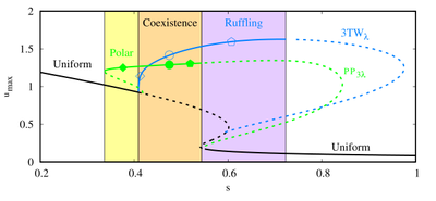
This model suite explores how cell shapes and motility are regulated by the negative feedback rate ($s$) and the cell perimeter ($L$) of a mass-conserved reaction-diffusion partial differential equation (PDE) model. Guided by numerical PDE bifurcation analysis, we couple the reaction-diffusion equations on the 1D cell perimeter to a 2D Cellular Potts model (CPM) to simulate various cell states, including directed motion, edge-ruffling, wobbly oscillations, back-and-forth turning, and random amoeboid-like motility.
Reproducibility of Article Figures
The Morpheus XML files for each of these models are provided directly on this page for simulation in the Morpheus GUI. For the complete computational pipeline, including Python analysis scripts, Jupyter notebooks, and the raw simulated cell trajectory data, please visit the GitLab repository.
Mathematical Model
We model the cell perimeter as a 1D membrane domain where active GTPase ($u$), inactive GTPase ($v$), and filamentous actin ($F$) evolve under reaction-diffusion dynamics:
$$ \frac{\partial u}{\partial t} = (b + \gamma u^2) v - (1 + u^2 + s F) u + D_u \frac{\partial^2 u}{\partial x^2} $$
$$ \frac{\partial v}{\partial t} = -(b + \gamma u^2) v + (1 + u^2 + s F) u + D_v \frac{\partial^2 v}{\partial x^2} $$
$$ \frac{\partial F}{\partial t} = \epsilon (p_0 + p_1 u - F) + D_F \frac{\partial^2 F}{\partial x^2} $$
Where:
- $u$ represents the active form of a GTPase (e.g. RhoA or Rac) bound to the membrane.
- $v$ represents the inactive cytosolic form.
- $F$ represents the F-actin downstream effector.
- $s$ is the F-actin-dependent GTPase inactivation rate (negative feedback rate).
- $b$ and $\gamma$ represent basal and auto-activation rates respectively.
- $\epsilon$, $p_0$, and $p_1$ govern F-actin assembly and disassembly rates.
- $D_u$, $D_v$, and $D_F$ are the respective diffusion coefficients on the cell perimeter.
The local value of F-actin ($F$) along the cell boundary is coupled to the CPM, favoring local membrane protrusions where $F$ is high, driving cell deformation and motility.
Motility Phenotypes and Simulations
1. Polar Cells (Directed Migration)
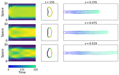
When parameter values lie on the stable unipolar branch, the cell maintains a single, stable peak of active GTPase. This concentrates F-actin at the cell front and drives persistent, directed migration.
- Simulation files:
polar_s_0.376.xml,polar_s_0.475.xml,polar_s_0.519.xml - Key behavior: As $s$ increases, the GTPase zone at the front narrows and active GTPase becomes more highly concentrated, increasing F-actin levels and propelling the cell faster (Figure 2).
2. Edge-Ruffling Cells (3 Traveling Waves)
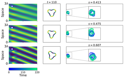
Along the traveling wave branch, multiple peaks can propagate along the perimeter.
- Simulation files:
tw_s_0.413.xml,tw_s_0.475.xml,tw_s_0.607.xml - Key behavior: The cell perimeter supports three traveling waves, creating three competing protrusions. Because the forces pull in opposite directions, the cell undergoes no directed migration, displaying a ruffling phenotype.
3. Destabilized Polar Cells (Wobbly Motion)
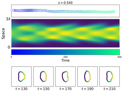
Just after the onset of polar pattern instability, the spatial pattern of GTPase oscillates periodically.
- Simulation file:
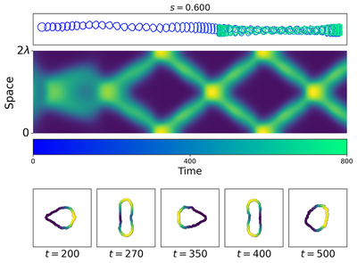
Wobby_s_0.600.xml(s = 0.54) - Key behavior: The active GTPase zone remains localized in one direction, maintaining directed motion, but oscillates in shape and concentration. This causes the cell shape to shift periodically between oval, D-like, and kidney shapes, and its migration speed fluctuates (Figure 4).
4. Coexisting Motility Modes & Exotic Trajectories
For smaller cells ($L = 2\lambda$), multiple modes can coexist and interact dynamically.
- Simulation files:
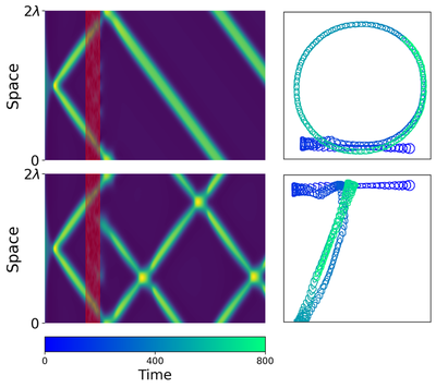
CW_s_0.600.xml,CW_s_0.8_noise.xml - Key behavior: At $s = 0.6$, the cell supports counter-propagating waves, moving back and forth (Figure 5). At $s = 0.8$, adding noise can disrupt one of the counter-propagating peaks, leaving a single traveling wave that leads to small circular turning paths or reversal of motion (Figure 6).
5. Transitions under Time-Dependent Feedback
By sweeping the negative feedback parameter $s(t)$ dynamically in time, cells can be driven across parity-breaking bifurcations.
- Simulation files:
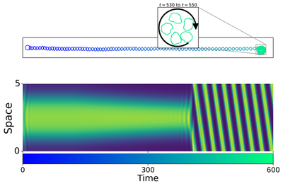
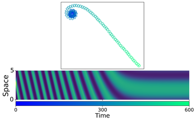
POLAR2TW_main.xml(directed to turning),TW2POLAR.xml(turning to directed) - Key behavior: A linear increase in $s$ causes a polar cell to transition into a single traveling wave and start turning (Figure 7). A linear decrease in $s$ brings the cell back from turning to directed migration (Figure 8).
6. Random Motion
- Simulation file:
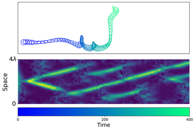
Random_motion.xml - Key behavior: By allowing $s(t)$ to undergo a random walk (Wiener process with reflective boundaries in the range $[0.475, 0.6]$), the cell transitions randomly between polar, counter-propagating peaks, and traveling waves, generating irregular trajectories.
![**Figure 9.** Cell motility under a randomly changing feedback parameter $s(t)$ executing a random walk in the range $[0.475, 0.6]$. The cell exhibits random switching between directed polar migration, counter-propagating peaks, and traveling waves.](/media/model/m2074/Fig14_hud5ba05a605f7631a0b53ca09c5352115_935365_cde1f63c5284fc0e3cf935af927836fc.png)
7. Continual Space-Time Noise
- Simulation file:
Dicty.xml - Key behavior: In larger cells ($L = 4\lambda$) with $s = 0.8$, continual space-time noise disrupts regular traveling waves. This leads to competing pseudopods where one randomly dominates the other, producing amoeboid-like motility trajectories that resemble Dictyostelium discoideum.
Reference
This model is the original used in the publication, up to technical updates:
J. M. Hughes, J. Algorta, L. Edelstein-Keshet: How negative feedback from filamentous actin affects cell shapes and motility. arXiv 2602.08779, 2026.
The model originates from a preprint and thus has not been formally peer-reviewed.
Model
POLAR2TW_main.xml
XML Preview
<MorpheusModel version="4">
<Description>
<Title>M2074 Transition from Directed Cell Motion to Cell Turning</Title>
<Details>Model ID: https://identifiers.org/morpheus/M2074
File type: Main model
Software: Morpheus (open source). Download from: https://morpheus.gitlab.io
Full title: How Negative Feedback from Filamentous Actin Affects Cell Shapes and Motility
Authors: J. M. Hughes, J. Algorta, L. Edelstein-Keshet
Submitter: J. Algorta
Curator: D. Jahn
Date: 07.06.2026
Reference: This model is the original used in the publication, up to technical updates:
J. M. Hughes, J. Algorta, L. Edelstein-Keshet: How negative feedback from filamentous actin affects cell shapes and motility. arXiv 2602.08779, 2026.
https://doi.org/10.48550/arXiv.2602.08779
Comment: This model simulates the transition from directed cell motion to cell turning due to a linearly increasing negative feedback rate s(t), simulated in Morpheus for Figure 12 of the publication. PDE model for F-actin negative feedback to GTPases, and GTPase promotion of F-actin. The reaction-diffusion PDEs are implemented on the cell edge. u = active GTPase (Rac), v = inactive GTPase, F = F-actin.</Details>
</Description>
<Global>
<Constant symbol="lengthscale" value="L/(2*sqrt(targetVol*pi))"/>
<Constant symbol="L" value="5"/>
<Constant symbol="targetVol" value="4800/2"/>
<Field symbol="prot" value="0.0"/>
<Variable symbol="time_var" value="0.0"/>
<System solver="Dormand-Prince [adaptive, O(5)]">
<Rule symbol-ref="time_var">
<Expression>time</Expression>
</Rule>
</System>
<Constant symbol="s0" value="0.475"/>
<Constant symbol="sf" value="0.6"/>
<Constant symbol="tf" value="500"/>
<Variable symbol="s" value="0.0"/>
<!-- <Disabled>
<Variable symbol="td" value="-ln(rand_uni(0,1))/lambda"/>
</Disabled>
-->
<!-- <Disabled>
<Variable symbol="lambda" value="20"/>
</Disabled>
-->
<Constant symbol="delta_size" value="0.005"/>
<Constant symbol="lambda" value="6*0.0001/(delta_size^2)"/>
</Global>
<Space>
<Lattice class="square">
<Size symbol="lattice" value="5000,5000, 0"/>
<!-- <Disabled>
<Size symbol="lattice" value="800/sqrt(2), 2*400/sqrt(2), 0"/>
</Disabled>
-->
<BoundaryConditions>
<Condition type="noflux" boundary="x"/>
<Condition type="noflux" boundary="y"/>
</BoundaryConditions>
<NodeLength value="1.0"/>
<Neighborhood>
<Distance>2.0</Distance>
</Neighborhood>
</Lattice>
<SpaceSymbol symbol="l"/>
<MembraneLattice>
<Resolution symbol="memsize" value="500"/>
<SpaceSymbol symbol="m"/>
</MembraneLattice>
</Space>
<Time>
<StartTime value="0"/>
<StopTime value="600"/>
<SaveInterval value="0"/>
<!-- <Disabled>
<RandomSeed value="0"/>
</Disabled>
-->
<TimeSymbol symbol="time"/>
</Time>
<CellTypes>
<CellType name="cells" class="biological">
<VolumeConstraint target="targetVol" strength="1" name=""/>
<SurfaceConstraint target="1.2" strength="1" mode="aspherity"/>
<MembraneProperty symbol="Noise" value="0.0">
<Diffusion well-mixed="false" rate="0.0"/>
</MembraneProperty>
<MembraneProperty symbol="u" name="Active form of protein" value="0.75-0.5*cos(m.phi)">
<Diffusion rate="0.1/lengthscale^2"/>
</MembraneProperty>
<MembraneProperty symbol="v" name="Inactive form of protein" value="1.25+0.1*cos(m.phi)">
<Diffusion rate="1/lengthscale^2"/>
</MembraneProperty>
<MembraneProperty symbol="F" name="F-actin" value="3.5-2*cos(m.phi)">
<Diffusion rate="0.001/lengthscale^2"/>
</MembraneProperty>
<Property symbol="s" value="s0"/>
<System time-scaling="1" time-step="0.05" name="WavePinning with Inhibitor" solver="Runge-Kutta [fixed, O(4)]">
<Constant symbol="b" value="0.067"/>
<Constant symbol="gamma" value="3.557"/>
<!-- <Disabled>
<Constant symbol="s" value="s0*(time < 1/4*tf)+ (s0-(s0-sf)*(time-1/4*tf)/(3/4*tf))*(time > 1/4*tf)*(time < tf)+sf*(time >tf)"/>
</Disabled>
-->
<Constant symbol="eps" value="0.6"/>
<Constant symbol="p0" value="0.8"/>
<Constant symbol="p1" value="3.8"/>
<Intermediate symbol="A" value="(b+gamma*u^2)*v-(1+s*F+u^2)*u"/>
<DiffEqn symbol-ref="u">
<Expression>A</Expression>
</DiffEqn>
<DiffEqn symbol-ref="v">
<Expression>-A</Expression>
</DiffEqn>
<DiffEqn symbol-ref="F">
<Expression>eps*(p0+p1*u-F)</Expression>
</DiffEqn>
<Rule symbol-ref="Noise">
<Expression>4*(time_var>150)*(time_var<200)*rand_norm(0,1)</Expression>
</Rule>
<!-- <Disabled>
<Rule symbol-ref="s">
<Expression>s0*(time < 1/4*tf)+ (s0-(s0-sf)*(time-1/4*tf)/(3/4*tf))*(time > 1/4*tf)*(time < tf)+sf*(time >tf)</Expression>
</Rule>
</Disabled>
-->
</System>
<System solver="Dormand-Prince [adaptive, O(5)]">
<Rule symbol-ref="s">
<Expression>s0*(time < 0.25*tf) + (s0-(s0-sf)*(time-0.25*tf)/(0.5*tf))*(time > 0.25*tf)*(time < 0.75*tf) + sf*(time > 0.75*tf)</Expression>
</Rule>
</System>
<StarConvex membrane="F" strength="1" retraction="false" protrusion="true"/>
<Protrusion strength="1" field="prot" maximum="150"/>
<!-- <Disabled>
<Event>
<Condition>(time > 1/4*tf)*(time < tf)</Condition>
<Rule symbol-ref="s">
<Expression>s0-(s0-sf)*(time-1/4*tf)/(3/4*tf)</Expression>
</Rule>
</Event>
</Disabled>
-->
<!-- <Disabled>
<Event>
<Condition>time > tf</Condition>
<Rule symbol-ref="s">
<Expression>sf</Expression>
</Rule>
</Event>
</Disabled>
-->
</CellType>
</CellTypes>
<CPM>
<Interaction default="0.0"/>
<MonteCarloSampler stepper="edgelist">
<MCSDuration value="0.01"/>
<Neighborhood>
<Order>2</Order>
</Neighborhood>
<MetropolisKinetics yield="0.05" temperature="1"/>
</MonteCarloSampler>
<ShapeSurface scaling="norm">
<Neighborhood>
<Order>6</Order>
</Neighborhood>
</ShapeSurface>
</CPM>
<CellPopulations>
<Population type="cells" size="0">
<InitCellObjects mode="distance">
<Arrangement repetitions="1, 1, 0" displacements="1, 1, 0">
<!-- <Disabled>
<Sphere center="2766 282 0" radius="24*2"/>
</Disabled>
-->
<Sphere center="4900 2000 0" radius="24*2"/>
</Arrangement>
</InitCellObjects>
</Population>
</CellPopulations>
<Analysis>
<Logger time-step="1">
<Input>
<Symbol symbol-ref="m.phi"/>
<Symbol symbol-ref="u"/>
<Symbol symbol-ref="F"/>
</Input>
<Output>
<TextOutput/>
</Output>
<Plots>
<Plot time-step="5">
<Style style="points"/>
<Terminal terminal="png"/>
<X-axis maximum="6.28">
<Symbol symbol-ref="m.phi"/>
</X-axis>
<Y-axis maximum="10">
<Symbol symbol-ref="u"/>
<Symbol symbol-ref="v"/>
<Symbol symbol-ref="F"/>
<!-- <Disabled>
<Symbol symbol-ref="Noise"/>
</Disabled>
-->
</Y-axis>
<Range>
<Time mode="current"/>
</Range>
</Plot>
<!-- <Disabled>
<SurfacePlot time-step="10">
<Color-bar>
<Symbol symbol-ref="u"/>
</Color-bar>
<Terminal terminal="png"/>
</SurfacePlot>
</Disabled>
-->
<Plot time-step="-1">
<Style style="points" point-size="1"/>
<Terminal terminal="png"/>
<X-axis>
<Symbol symbol-ref="time"/>
</X-axis>
<Y-axis minimum="0.0" maximum="6.3">
<Symbol symbol-ref="m.phi"/>
</Y-axis>
<Color-bar>
<Symbol symbol-ref="u"/>
</Color-bar>
</Plot>
<Plot time-step="5">
<Style style="points"/>
<Terminal terminal="png"/>
<X-axis>
<Symbol symbol-ref="time"/>
</X-axis>
<Y-axis>
<Symbol symbol-ref="s"/>
</Y-axis>
</Plot>
<!-- <Disabled>
<Plot time-step="-1">
<Style style="points"/>
<Terminal terminal="png"/>
<X-axis>
<Symbol symbol-ref="time"/>
</X-axis>
<Y-axis>
<Symbol symbol-ref="s"/>
</Y-axis>
</Plot>
</Disabled>
-->
</Plots>
</Logger>
<ModelGraph include-tags="#untagged" format="dot" reduced="false"/>
<Gnuplotter time-step="5" decorate="false" log-commands="true">
<Plot>
<Cells value="F"/>
<!-- <Disabled>
<Field symbol-ref="prot"/>
</Disabled>
-->
</Plot>
<Terminal name="png" size="1200,1200,0"/>
</Gnuplotter>
<!-- <Disabled>
<Logger time-step="-1">
<Input>
<Symbol symbol-ref="cell.center.x"/>
<Symbol symbol-ref="cell.center.y"/>
</Input>
<Output>
<TextOutput/>
</Output>
<Plots internal:disabled="true">
<Plot time-step="-1">
<Style style="points" point-size="0.5"/>
<Terminal terminal="png"/>
<X-axis>
<Symbol symbol-ref="cell.center.x"/>
</X-axis>
<Y-axis>
<Symbol symbol-ref="cell.center.y"/>
</Y-axis>
<Color-bar>
<Symbol symbol-ref="time"/>
</Color-bar>
</Plot>
</Plots>
</Logger>
</Disabled>
-->
<!-- <Disabled>
<Gnuplotter time-step="20" decorate="false" log-commands="true">
<Plot>
<Cells value="cell.id"/>
</Plot>
<Terminal name="png"/>
</Gnuplotter>
</Disabled>
-->
<CellTracker time-step="1.0" format="ISBI 2012 (XML)"/>
<Logger time-step="0.1">
<Input>
<Symbol symbol-ref="s"/>
<!-- <Disabled>
<Symbol symbol-ref="cell.center.y"/>
</Disabled>
-->
</Input>
<Output>
<TextOutput/>
</Output>
<Plots>
<!-- <Disabled>
<Plot time-step="-1">
<Style style="points" point-size="0.5"/>
<Terminal terminal="png"/>
<X-axis>
<Symbol symbol-ref="cell.center.x"/>
</X-axis>
<Y-axis>
<Symbol symbol-ref="cell.center.y"/>
</Y-axis>
<Color-bar>
<Symbol symbol-ref="time"/>
</Color-bar>
</Plot>
</Disabled>
-->
<Plot time-step="-1">
<Style style="points"/>
<Terminal terminal="png"/>
<X-axis>
<Symbol symbol-ref="time"/>
</X-axis>
<Y-axis>
<Symbol symbol-ref="s"/>
</Y-axis>
</Plot>
</Plots>
</Logger>
<Logger time-step="1">
<Input>
<Symbol symbol-ref="m.phi"/>
<!-- <Disabled>
<Symbol symbol-ref="u"/>
</Disabled>
-->
<Symbol symbol-ref="F"/>
</Input>
<Output>
<TextOutput/>
</Output>
<!-- <Disabled>
<Plots>
<Plot time-step="5" internal:disabled="true">
<Style style="points"/>
<Terminal terminal="png"/>
<X-axis maximum="6.28">
<Symbol symbol-ref="m.phi"/>
</X-axis>
<Y-axis maximum="10">
<Symbol symbol-ref="u"/>
<Symbol symbol-ref="v"/>
<Symbol symbol-ref="F"/>
<Symbol symbol-ref="Noise" internal:disabled="true"/>
</Y-axis>
<Range>
<Time mode="current"/>
</Range>
</Plot>
<SurfacePlot time-step="10" internal:disabled="true">
<Color-bar>
<Symbol symbol-ref="u"/>
</Color-bar>
<Terminal terminal="png"/>
</SurfacePlot>
<Plot time-step="-1" internal:disabled="true">
<Style style="points" point-size="1"/>
<Terminal terminal="png"/>
<X-axis>
<Symbol symbol-ref="time"/>
</X-axis>
<Y-axis minimum="0.0" maximum="6.3">
<Symbol symbol-ref="m.phi"/>
</Y-axis>
<Color-bar>
<Symbol symbol-ref="u"/>
</Color-bar>
</Plot>
<Plot time-step="5" internal:disabled="true">
<Style style="points"/>
<Terminal terminal="png"/>
<X-axis>
<Symbol symbol-ref="time"/>
</X-axis>
<Y-axis>
<Symbol symbol-ref="s"/>
</Y-axis>
</Plot>
<Plot time-step="-1" internal:disabled="true">
<Style style="points"/>
<Terminal terminal="png"/>
<X-axis>
<Symbol symbol-ref="time"/>
</X-axis>
<Y-axis>
<Symbol symbol-ref="s"/>
</Y-axis>
</Plot>
</Plots>
</Disabled>
-->
</Logger>
</Analysis>
</MorpheusModel>
Model Files Included
Main Model Configurations
POLAR2TW_main.xml: Transition from directed motion to turning (increasing $s(t)$, Figure 12)TW2POLAR.xml: Transition from turning to directed motion (decreasing $s(t)$, Figure 13)CW_s_0.600.xml: Coexisting back-and-forth motility ($s = 0.600, L = 2\lambda$, Figure 10)CW_s_0.8_noise.xml: Exotic trajectories under noise ($s = 0.800, L = 2\lambda$, Figure 11)Wobby_s_0.600.xml: Wobbly shape and speed oscillations ($s = 0.540$, Figure 9)Random_motion.xml: Random motion under fluctuating parameter $s(t)$ (Figure 14)Dicty.xml: Amoeboid-like motility with continual noise ($s = 0.800, L = 4\lambda$, Figure 16)
Polar Cell Motility Branch (Figure 7)
polar_s_0.376.xml: Polar cell state at $s = 0.376$polar_s_0.475.xml: Polar cell state at $s = 0.475$polar_s_0.519.xml: Polar cell state at $s = 0.519$
Traveling Wave Ruffling Cell Branch (Figure 8)
tw_s_0.413.xml: Edge-ruffling cell state at $s = 0.413$tw_s_0.475.xml: Edge-ruffling cell state at $s = 0.475$tw_s_0.607.xml: Edge-ruffling cell state at $s = 0.607$
Downloads
Files associated with this model:
CW_s_0.600.xmlCW_s_0.8_noise.xmlDicty.xmlFig10.pngFig11.pngFig12.pngFig13.pngFig14.pngFig16.pngFig5.pngFig7.pngFig8.pngFig9.pngm2074_f-actin-feedback-in-cell-motility_model-graph.svgPOLAR2TW_main.xmlpolar_s_0.376.xmlpolar_s_0.475.xmlpolar_s_0.519.xmlRandom_motion.xmlTW2POLAR.xmltw_s_0.413.xmltw_s_0.475.xmltw_s_0.607.xmlWobby_s_0.600.xml