Eukaryotic Cell Motility Based on Actin Waves on the Cell Edge
Persistent Identifier
Use this permanent link to cite or share this Morpheus model:
Cell motility simulation with a reaction-diffusion model for actin waves on the cell perimeter
Introduction
A partial differential equation model for ‘actin waves’ by Holmes et al., 2012 was simplified and investigated by PDE bifurcation analysis in Hughes et al., 2024.
This model is related to our model of actin waves in 1D and our previous work Mata et al., 2013 and Liu et al., 2021.
Description
The model accounts for active ($u$) and inactive ($v$) GTPase (such as Rac) and its nucleation of filamentous actin ($F$). We assumed that Rac promotes F-actin assembly, and that F-actin contributes negative feedback (inactivation of Rac).
The model equations are:
$$\begin{align} \frac{\partial u}{\partial t} &= (b+\gamma u^2)v - (1+sF+u^2)u + D \Delta u \\ \frac{\partial v}{\partial t} &= -(b+\gamma u^2)v + (1+sF+u^2)u + \Delta v \\ \frac{\partial F}{\partial t} &= \epsilon (p_0+p_1 u - F) + D_F \Delta F \end{align}$$
The dynamics of these equations in a 1D periodic domain, and XML files for simulating the model are given on model page M2071.
Here we investigate the effect of ‘actin wave’ dynamics on the protrusion and motility of a eukaryotic cell.
We assumed that the reaction-diffusion model operates on the 1D periodic cell-edge domain of a CPM cell. Using the Morpheus plugin StarConvex membrane based on the level of F-actin ($F$), we simulated the PDEs as a MembraneProperty system for a single cell, with parameter values given in the table below.
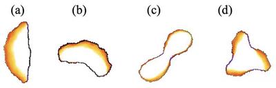
Two_Lobe_Cell.xml) and three-lobe (Three_Lobe_Cell.xml) configurations, the lengthscale parameter is set as described below, and all other parameters are as for the Turning Cell configuration.To observe distinct behaviors, we picked cells of ‘different sizes’: we used similar kinetic parameters, but changed the lengthscale.
The lengthscale was obtained by adjusting the diffusion coefficients: in the Polar Cell, this coefficient was set to $\frac{1}{5}$; in the Turning Cell, to $\frac{1}{100}$; in the two-lobe configuration, to $\frac{1}{50}$ (twice the Turning Cell coefficient); and in the three-lobe configuration, to $\frac{1}{33}$ (three times the Turning Cell coefficient).
Results
Cell shape and motility vary depending on the type of PDE solution, determined by the parameter values and domain size, $L$. Four qualitatively different motility states are compared in Figure 1 (a)-(d) and the associated Videos 1-4 below. For each case, the corresponding model file is linked in the video caption.
Polar_Cell_Motility_main.xml
Turning_Cell_Motility.xml
Two_Lobe_Cell.xml
Three_Lobe_Cell.xml
Reference
This model is the original used in the publication, up to technical updates:
J. Algorta, A. Fele-Paranj, J. M. Hughes, L. Edelstein-Keshet: Modeling and Simulating Single and Collective Cell Motility. Cold Spring Harb. Perspect. Biol., 2025.
Model
Polar_Cell_Motility_main.xml
XML Preview
<MorpheusModel version="4">
    <Description>
        <Title>M2072 Polar Cell Motility</Title>
        <Details>Model ID:	https://identifiers.org/morpheus/M2072
  File type:	Main model
  Software:	Morpheus (open source). Download from: https://morpheus.gitlab.io
Full title:	Eukaryotic Cell Motility – Polar Cell
Authors:	J. Algorta, A. Fele-Paranj, J. M. Hughes, L. Edelstein-Keshet
Submitter:	J. Algorta, L. Edelstein-Keshet
Curator:	D. Jahn
Date:	12.11.2024
Reference:	J. Algorta, A. Fele-Paranj, J. M. Hughes, L. Edelstein-Keshet: Modeling and Simulating Single and Collective Cell Motility. Cold Spring Harb. Perspect. Biol., 2025. https://doi.org/10.1101/cshperspect.a041796
	This model is the original used in Figure 2 of the publication, up to technical updates.
Comment:	PDE model for F-actin negative feedback to GTPases, and GTPase promotion of F-actin. The reaction-diffusion PDEs are implemented on the cell edge.
	u = active GTPase (Rac)
	v = inactive GTPase
	F = F-actin</Details>
    </Description>
    <Global>
        <Constant symbol="lengthscale" value="1/5"/>
        <Field symbol="prot" value="0.0"/>
    </Global>
    <Space>
        <Lattice class="square">
            <Size symbol="lattice" value="600, 600, 0"/>
            <BoundaryConditions>
                <Condition type="periodic" boundary="x"/>
                <Condition type="periodic" boundary="y"/>
            </BoundaryConditions>
            <NodeLength value="1.0"/>
            <Neighborhood>
                <Distance>2.0</Distance>
            </Neighborhood>
        </Lattice>
        <SpaceSymbol symbol="l"/>
        <MembraneLattice>
            <Resolution symbol="memsize" value="1500"/>
            <SpaceSymbol symbol="m"/>
        </MembraneLattice>
    </Space>
    <Time>
        <StartTime value="0"/>
        <StopTime value="400"/>
        <SaveInterval value="0"/>
        <!--    <Disabled>
        <RandomSeed value="0"/>
    </Disabled>
-->
        <TimeSymbol symbol="time"/>
    </Time>
    <CellTypes>
        <CellType class="biological" name="cells">
            <VolumeConstraint target="4800" strength="1"/>
            <SurfaceConstraint target="1.2" strength="1" mode="aspherity"/>
            <MembraneProperty symbol="u" name="Active form of protein" value="1-0.5*cos(m.phi)">
                <Diffusion rate="0.1/lengthscale^2"/>
            </MembraneProperty>
            <MembraneProperty symbol="v" name="Inactive form of protein" value="1-0.1*cos(m.phi)">
                <Diffusion rate="1/lengthscale^2"/>
            </MembraneProperty>
            <MembraneProperty symbol="F" name="F-actin" value="4.5-0.82*cos(m.phi)">
                <Diffusion rate="0.001/lengthscale^2"/>
            </MembraneProperty>
            <Constant symbol="T" value="0"/>
            <System time-step="0.05" name="WavePinning with Inhibitor" time-scaling="0.1" solver="Runge-Kutta [fixed, O(4)]">
                <Constant symbol="b" value="0.067"/>
                <Constant symbol="gamma" value="3.55"/>
                <Constant symbol="s" value="0.41"/>
                <Constant symbol="eps" value="0.6"/>
                <Constant symbol="p0" value="0.8"/>
                <Constant symbol="p1" value="3.8"/>
                <Intermediate symbol="A" value="(b+gamma*u^2)*v-(1+(s)*F+(1+trial*T)*u^2)*u"/>
                <DiffEqn symbol-ref="u">
                    <Expression>A</Expression>
                </DiffEqn>
                <DiffEqn symbol-ref="v">
                    <Expression>-A</Expression>
                </DiffEqn>
                <DiffEqn symbol-ref="F">
                    <Expression>eps*(p0+p1*u-F)</Expression>
                </DiffEqn>
                <Constant symbol="trial" value="0"/>
            </System>
            <StarConvex retraction="false" membrane="F" protrusion="true" strength="5"/>
            <Protrusion maximum="150" strength="10.5" field="prot"/>
        </CellType>
    </CellTypes>
    <CPM>
        <Interaction default="0.0"/>
        <MonteCarloSampler stepper="edgelist">
            <MCSDuration value="0.01"/>
            <Neighborhood>
                <Order>2</Order>
            </Neighborhood>
            <MetropolisKinetics yield="0.05" temperature="1"/>
        </MonteCarloSampler>
        <ShapeSurface scaling="norm">
            <Neighborhood>
                <Order>6</Order>
            </Neighborhood>
        </ShapeSurface>
    </CPM>
    <CellPopulations>
        <Population type="cells" size="0">
            <InitCellObjects mode="distance">
                <Arrangement displacements="1, 1, 0" repetitions="1, 1, 0">
                    <Sphere radius="24*2" center="400 200 0"/>
                </Arrangement>
            </InitCellObjects>
        </Population>
    </CellPopulations>
    <Analysis>
        <Logger time-step="10">
            <Input>
                <Symbol symbol-ref="m.phi"/>
                <Symbol symbol-ref="u"/>
                <Symbol symbol-ref="T"/>
                <Symbol symbol-ref="F"/>
            </Input>
            <Output>
                <TextOutput/>
            </Output>
            <Plots>
                <Plot time-step="10">
                    <Style style="points"/>
                    <Terminal terminal="png"/>
                    <X-axis maximum="6.28">
                        <Symbol symbol-ref="m.phi"/>
                    </X-axis>
                    <Y-axis maximum="10">
                        <Symbol symbol-ref="u"/>
                        <Symbol symbol-ref="v"/>
                        <Symbol symbol-ref="F"/>
                    </Y-axis>
                    <Range>
                        <Time mode="current"/>
                    </Range>
                </Plot>
            </Plots>
        </Logger>
        <ModelGraph format="dot" reduced="false" include-tags="#untagged"/>
        <Gnuplotter time-step="5" decorate="false">
            <Plot>
                <Cells value="F"/>
                <Field symbol-ref="prot"/>
            </Plot>
            <Terminal name="png" size="1200,1200,0"/>
            <!--    <Disabled>
        <Plot/>
    </Disabled>
-->
        </Gnuplotter>
    </Analysis>
</MorpheusModel>

Downloads
Files associated with this model:
M2072_eukaryotic-cell-motility_fig-1_cell-shapes.jpgM2072_eukaryotic-cell-motility_model-graph.svgPolar_Cell_Motility_main.xmlPolar_Cell_Motility_movie.mp4Three_Lobe_Cell.xmlThree_Lobe_Cell_movie.mp4Turning_Cell_Motility.xmlTurning_Cell_Motility_movie.mp4Two_Lobe_Cell.xmlTwo_Lobe_Cell_movie.mp4