Simplified Actin Waves in Eukaryotic Cell Motility

J. Algorta, A. Fele-Paranj, J. M. Hughes, L. Edelstein-Keshet (Authors)

J. M. Hughes, L. Edelstein-Keshet (Contributors)

Persistent Identifier

Use this permanent link to cite or share this Morpheus model:

Spatial relaxation oscillator produces spatial dynamics and spiral waves, simplification of a previous model for actin waves

Introduction

Motivated by alternative cell motility modes in eukaryotic cells like Dictyostelium discoideum, we consider a simplified version of an intracellular model for an F-actin negative feedback to an (active/inactive) GTPase system. The equations were analysed by full PDE bifurcation analysis in Hughes et al., 2024.

Description

This model is related to a previous model on actin waves.

Equations: for the active ($u$), inactive ($v$) GTPase, respectively, and F-actin ($F$).

$$\begin{align} \frac{\partial u}{\partial t} &= (b+\gamma u^2)v - (1+sF+u^2)u + D \Delta u \\ \frac{\partial v}{\partial t} &= -(b+\gamma u^2)v + (1+sF+u^2)u + \Delta v \\ \frac{\partial F}{\partial t} &= \epsilon (p_0+p_1 u - F) + D_F \Delta F \end{align}$$

The domain is periodic, of (side) length $L$, in 1D and 2D.

The parameters and initial conditions are given in the following table.

		Polar 1D	Traveling Waves 1D	Spiral Waves
Params.	$b$	$0.067$	$0.067$	$1.5$
	$\gamma$	$3.55$	$3$	$30$
	$s$	$0.41$	$1$	$10$
	$\epsilon$	$0.6$	$0.6$	$0.6$
	$p_0$	$0.8$	$0.8$	$0.8$
	$p_1$	$3.8$	$3.8$	$3.8$
	$D$	$0.1$	$0.1$	$0.1$
	$D_F$	$0.001$	$0.001$	$0.001$
	$M$	$2$	$4.5$	$3$
	$L$	$2\pi$	$pi$	$10$
Initial conditions		$\begin{align}\scriptsize u(x, 0) \ &\scriptsize= 1 - 0.5 \cos(x)\\ \scriptsize v(x, 0) \ &\scriptsize= 1 - 0.1 \cos(x)\\ \scriptsize F(x, 0) \ &\scriptsize= 4.5 - 0.82 \cos(x)\end{align}$	$\begin{align}\scriptsize u(x, 0) \ &\scriptsize= 1 - 0.5 \cos(x) - 0.6 \sin(x)\\ \scriptsize v(x, 0) \ &\scriptsize= 1 - 0.1 \sin(x)\\ \scriptsize F(x, 0) \ &\scriptsize= 4.5 - 0.82 \cos(x)\end{align}$	$\begin{align}\scriptsize u(x, 0) \ &\scriptsize= 0.5\\ \scriptsize v(x, 0) \ &\scriptsize= M - 0.5 \scriptsize= 2.5\\ \scriptsize F(x, 0) \ &\scriptsize= 4.5 + \chi\end{align}$
Model file		`ActinWavesPDE 1DPolar_main.xml`	`ActinWavesPDE 1DTW.xml`	`ActinWavesPDE 2DSpiral.xml`

Table 1: Parameters and initial conditions. Where, for the spiral waves, $\chi = 0.7(0.5 − \sigma)$ for $\sigma$ a normally distributed random number between $[−0.5, 0.5]$, which is adding noise to the initial condition.

Results

One-dimensional analysis

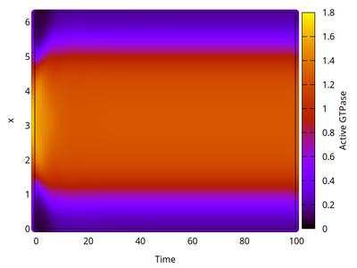
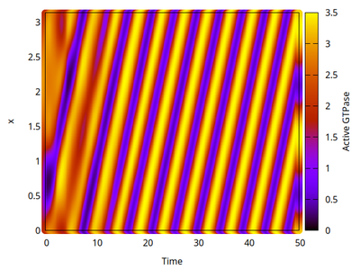
In 1D spatial coordinates we obtain either a polar distribution or a traveling wave, as shown for the variable $u$ in the two kymographs below. Time evolves (horizontal axis) and space is on the vertical axis.

Kymograph of 1D model simulation shows stationary polarized state — **Figure 1:** Kymograph of 1D model simulation, with parameters of first column in above table and periodic boundary conditions, shows a **stationary polarized state**.

Kymograph of 1D model simulation shows traveling wave — **Figure 2:** Kymograph of 1D model simulation, with parameters of second column in above table and periodic boundary conditions, shows a **traveling wave** with one active domain.

Two-dimensional analysis

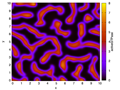
In 2D spatial coordinates, the system can also form dynamic spiral waves as shown in the snapshot and movie below.

Snapshot of 2D model simulation shows spiral waves — **Figure 3:** Snapshot of 2D model simulation, with parameters of third column in above table and periodic boundary conditions, shows **spiral waves**.

Reference

This model is the original used in the publication, up to technical updates:

J. Algorta, A. Fele-Paranj, J. M. Hughes, L. Edelstein-Keshet: Modeling and Simulating Single and Collective Cell Motility. Cold Spring Harbour Perspectives in Biology, 2024.

Model

Get this model via:

Morpheus-Link or

Download: ActinWavesPDE1DPolar_main.xml

XML Preview

<MorpheusModel version="4">
    <Description>
        <Title>Actin WavesHughesPolar1D</Title>
        <Details>Model ID:	https://identifiers.org/morpheus/M2071
  File type:	Main model
  Software:	Morpheus (open source). Download from: https://morpheus.gitlab.io
Full title:	Simplified Actin Waves in Eukaryotic Cell Motility – Polar 1D
Authors:	J. M. Hughes and L. Edelstein-Keshet 
Submitter:	L. Edelstein-Keshet
Curator:	D. Jahn
Date:	29.10.2024
Reference:	J. Algorta, A. Fele-Paranj, J. M. Hughes, L. Edelstein-Keshet: Modeling and Simulating Single and Collective Cell Motility. Cold Spring Harbour Perspectives in Biology, 2024.
	This model reproduces the model and results obtained with Morpheus in Figure 1 of the original publication.
Comment:	PDE model for F-actin negative feedback to GTPases, and GTPase promotion of F-actin.
	u = active GTPases
	v = inactive GTPase
	F = F-actin</Details>
    </Description>
    <!--
 Define the variables and initialize their values.
 Indicate the rates of diffusion
 GTPases diffusem but F-actin does not
-->
    <Global>
        <Field symbol="u" name="Active GTPase" value="1-0.5* cos(x)">
            <Diffusion rate="0.1/dx/dx"/>
        </Field>
        <Field symbol="v" name="Inactive GTPase" value="1-0.1* cos(x)">
            <Diffusion rate="1/dx/dx"/>
        </Field>
        <Field symbol="F" name="F-actin" value="4.5 + 0.82* cos(x)">
            <Diffusion rate="0.001/dx/dx"/>
        </Field>
        <!--
 Specify the method of solution and give the kinetic terms
 in the differential equations for the three variables
-->
        <System time-step="0.05" solver="Dormand-Prince [adaptive, O(5)]">
            <DiffEqn symbol-ref="u">
                <Expression> (b+gamma*u^n)*v- u*(1+s*F+u^2) </Expression>
            </DiffEqn>
            <DiffEqn symbol-ref="v">
                <Expression> -(b+gamma*u^n)*v+ u*(1+s*F+u^2) </Expression>
            </DiffEqn>
            <DiffEqn symbol-ref="F">
                <Expression> epsilon*(p0+p1*u-F)</Expression>
            </DiffEqn>
            <!--
  Define the constants and give their values.
-->
            <Constant symbol="b" name="basal activation rate" value="0.067"/>
            <Constant symbol="gamma" name="autocatalytic activation rate" value="3.55"/>
            <Constant symbol="n" name="Hill coefficient" value="2"/>
            <Constant symbol="p1" name="GTPase dependent F-actin assembly rate" value="3.8"/>
            <Constant symbol="p0" name="F-actin basal growth rate" value="0.8"/>
            <Constant symbol="s" name="actin-dependent GTPase inactivation rate" value="0.41"/>
            <Constant symbol="epsilon" name="actin reaction rate" value="0.6"/>
        </System>
        <Function symbol="x">
            <Expression>dx*space.x</Expression>
        </Function>
        <Constant symbol="dx" value="0.02"/>
    </Global>
    <!--
Specify the 2D Domain ("Square" lattice) and its boundary conditions
Indicate the size of each spatial box
-->
    <Space>
        <Lattice class="linear">
            <Size symbol="size" value="314, 0, 0"/>
            <BoundaryConditions>
                <Condition type="periodic" boundary="x"/>
                <!--    <Disabled>
        <Condition type="periodic" boundary="y"/>
    </Disabled>
-->
            </BoundaryConditions>
            <Neighborhood>
                <Order>1</Order>
            </Neighborhood>
        </Lattice>
        <SpaceSymbol symbol="space"/>
    </Space>
    <!--
  Set the start and end time and any random seed needed
-->
    <Time>
        <StartTime value="0"/>
        <StopTime value="100"/>
        <SaveInterval value="0"/>
        <TimeSymbol symbol="time"/>
    </Time>
    <!--
 Specify how the results should be plotted
-->
    <Analysis>
        <Logger time-step="0.1">
            <Input>
                <Symbol symbol-ref="u"/>
                <Symbol symbol-ref="v"/>
                <Symbol symbol-ref="F"/>
                <Symbol symbol-ref="x"/>
            </Input>
            <Output>
                <TextOutput file-format="csv"/>
            </Output>
            <Plots>
                <Plot time-step="20">
                    <Style point-size="2.0" style="points"/>
                    <Terminal terminal="png"/>
                    <X-axis minimum="0.0" maximum="100">
                        <Symbol symbol-ref="time"/>
                    </X-axis>
                    <Y-axis minimum="0.0" maximum="6.28">
                        <Symbol symbol-ref="x"/>
                    </Y-axis>
                    <Color-bar>
                        <Symbol symbol-ref="u"/>
                    </Color-bar>
                </Plot>
            </Plots>
        </Logger>
        <ModelGraph format="dot" reduced="false" include-tags="#untagged"/>
    </Analysis>
</MorpheusModel>

Downloads

Files associated with this model:

Last updated on Thu, 05 Dec 2024