Step-by-Step Example
To show SBML support in Morpheus as of version 2.1 in practice, we give a step-by-step example of how to download, import and extend an SBML model.
1. Get an SBML Model from BioModels
First, we browse the BioModels model repository and select a model.
In this case, we will browse the Gene Ontology annotation of the models and select a cell cycle model:
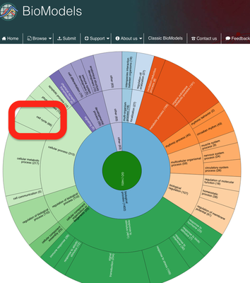
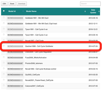
Here, we will use the cell cycle model described in Gardner et al. (1998) and choose it from the list:
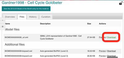
Next, under the ‘Files’ tab, we can download the SBML model and save the file BIOMD0000000008_url.xml to our Downloads directory:
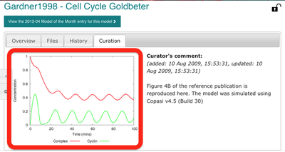
Under the ‘Curation’ tab, we can also have a look at a plot that was reproduced from the original publication using the SBML model:
2. Import SBML in Morpheus
Now that we have our SBML model, let us import it in Morpheus. To do this, click on Import SBML under the File menu item in the GUI.
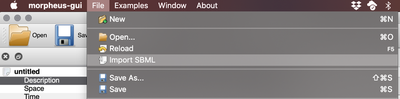
File → Import SBML.
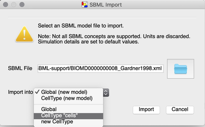
In the SBML import dialog that appears, we first locate our SBML model file. Then, we have several options to import the SBML model into a Morpheus model.
Importing the SBML model will create a System with e.g. variables, constants and differential equations containing all the model components. However, we can choose where to put that System.
We can create
- an entire new model or
- import it into an existing one, i.e. the currently selected model.
Also, we can choose to put it in
- the
Globalsection or - the
CellTypesection of the model.
If your model already contains a CellType, you can also import it into this existing CellType.
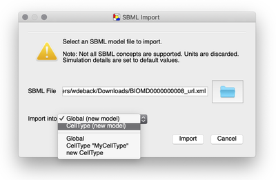
CellType is particularly useful if your aim is to extend the SBML model into a multicellular model.
Since we aim to extend the single cell model into a new multicellular model, we choose the CellType (new model) option and press Import.
Starting with Morpheus version 2.2, you can quickly and easily download, import and share SBML files using the Morpheus URL schema:
morpheus:///import?url=<URL>
In the case of our cell cycle model, the URL looks like this:
morpheus:///import?url=https://www.ebi.ac.uk/biomodels/model/download/BIOMD0000000008.2?filename=BIOMD000000000008_url.xml
Give it a try and open the import dialogue once more by clicking on this
Morpheus Link. Then, if you have already imported the model manually as described above, simply Cancel the window again.
3. Validate the SBML Model
During importing, a new model is created, the SBML model is translated into MorpheusML and appears as a System in a new CellType. Variables are renamed Property, RateRules are renamed as DiffEqn, FunctionDefinitionss become Functions etc.
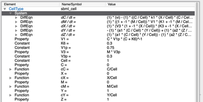
System in CellType.
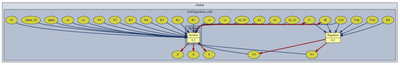
As in every Morpheus model, we can also look at the symbol dependency graph in Description:
Morpheus turns your SBML file into a simulation-ready model. However, some fields may need to be adjusted. Since simulation details such as the duration of simulation are not specified in the SBML model itself (rather, they are defined in an accompanying SED-ML file), Morpheus uses default values for this field. In this case, we can keep the default (Time/StopTime/value=100.0).
Morpheus also automatically defines the simulation output by configuring a Logger that keeps track of all model variables and creates a plot from them. This can be used to directly validate Morpheus.
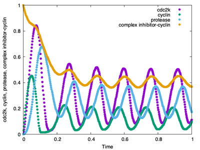
Thus, after importing, we can immediately run the model, obtain simulation results and validate the results against the curated plot from the BioModels repository:
 from the BioModels repository. For better visibility, we do not plot cyclin inhibitor (its symbol $Y$ is `Disabled` in the `Logger` plot).](/media/course/sbml-import/import-5_hu79776e308791152a8edf9798bad98ce5_105254_92c5ba5a6cad32ad3abbbdb896ace39a.png)
Disabled in the Logger plot).
4. Converting an Intracellular Model into a Multicellular Model
We could now extend this model into a multicellular CPM model by including a VolumeConstraint and SurfaceConstraint and add a CellDivision plugin whose Condition depends on some variable in the imported model. You’ll also need to use a 2D or 3D lattice in Space, add a spatial initializer such as InitCellObjects, specify your CPM model and visualize using a Gnuplotter.
However, let’s concentrate on a slightly different use case: Suppose you already have a multicellular model and now you want to include a different or a more realistic cell cycle model into this existing model. Here’s how:
As our base multicellular model, we’ll use the multiscale CellCycle.xml model.
Check out CellCycle.xml to try yourself via:
- Morpheus Link or
- Morpheus GUI:
Examples→Multiscale→CellCycle.xmlor - Morpheus Model Repository.
This model currently uses the cell cycle model by Ferrell et al. (2011), but we’ll replace it with the cell cycle model by Gardner et al. (1998), downloaded from BioModels.
After opening, you’ll see the model by Ferrell et al. (2011) in the CellType:
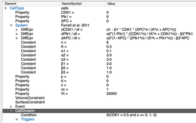
CellTypes section of the multiscale CellCycle.xml example model.
Now, we can add the cell cycle model from Gardner et al. (2008):
CellType ‘cells’ of the existing model.
As already practiced in step 2, there are two ways to import the SBML model:
- Use the
BIOMD0000000008_url.xmlfile you downloaded from the BioModels model page and navigate toFile→Import SBMLin the Morpheus GUI, or - import it directly by clicking on this Morpheus Link.
Afterwards, we can see that a new System with the Gardner model has been added, including a list of properties, constants, functions and differential equations. You have to manually comment out the previously used model:
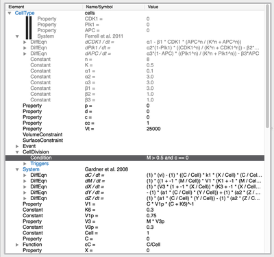
System with the Ferrell model above.
Now, to make cell division dependent on the new model, we need to change the CellType/CellDivision/Condition to depend on the value of M for cdc2k from the Gardner model instead of the CDK1 property in the Ferrell model (see highlighted line above). And the same for the Event that resets the variable c whenever M is low.
Additionally, we will need to adjust the Gnuplotter and Logger plugins to track the new Gardner variables instead of the Ferrell variables, and remove the InitProperty that specifies the initial condition for CDK1.
Once we’ve done that, we can run our model and observe this:
Tuning Time Scales
We forgot something important! If you look at the time course plot below, you’ll see that the cell cycle model has not yet completed a single cycle:
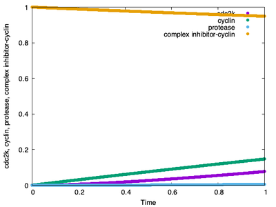
Logger time plot, which is created when the simulation run is finished, does not even show us a single completed cycle.
This is because the CellCycle.xml model is set to run from StartTime 0.0 to StopTime 1.0, while the Gardner model completes 6 cycles in 100 time units (see the Morpheus output for the imported Gardner model in step 3). Thus, the Ferrell CPM model and the Gardner ODE model operate on different time scales.
You can solve this by speeding up the System using the time-scaling option set to 100.0 as shown below.
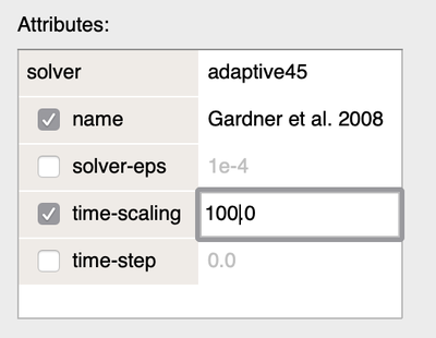
MetropolisKinetics/MCSDuration and run the simulation with StopTime=100.
After tuning the time scales between the ODE and CPM model, we obtain our cell cycle simulation with the Gardner model:
The associated time course plot now also looks as expected with the correct number of complete cycles.
time-scaling properly set, the Gardner model runs through 6 cycles again.