Try the Examples
Examples Menu
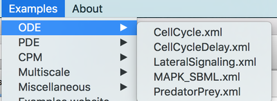
To explore the potential and modeling features, it is the best to learn by example. Morpheus comes with a range of fully functional example models showcasing a number of model formalism and modeling features. You can open these models from the Examples menu:
Examples menu try out some models.
There are models showing ordinary differential equations as well as reaction-diffusion systems in 1D, 2D and 3D and cell-based simulations with the cellular Potts model. Moreover, there are several multi-scale models in which the above models are combined and some other miscellaneous models.
 provided with Morpheus.](/media/course/getting-started/morpheus-gui-3_hud8bd96448bcebd9b6e9b8ba5fe8209cc_1037604_cae17cf40a7faa8bd52ad6d6dcdf1820.png)
We recommend that you have try out a few models, change parameters, add or remove some things, change the visualization, etc. to get a feel of what modeling with Morpheus is like.
Three Basic Models
We suggest that you take a look at the following three basic models. Just press run and pay attention to how the models are defined. Take the chance to change some parameters and see what happens.
ODE: Predator-Prey
This model implements an extension of the well-known Lotka-Volterra system.
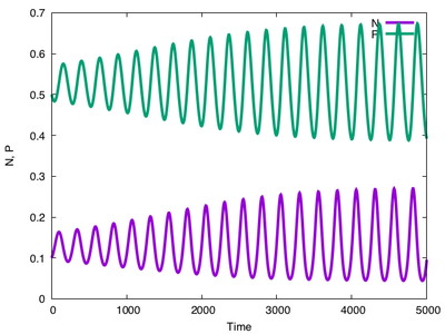
PredatorPrey.xml example model.
Check out PredatorPrey.xml to try yourself via:
- Morpheus Link or
- Morpheus GUI:
Examples→ODE→PredatorPrey.xmlor - Morpheus Model Repository.
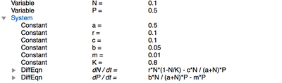
If you look at the model itself, you’ll see that it first specifies the Space and Time of a simulation, here defined as a single lattice site and $5000\ \mathrm{atu}$ (arbitrary time units). In Global (see figure below), two Variables for predator and prey densities are set up. The differential equations themselves are specified in a System which consists of a number of Constants and two DiffEqn (differential equations) and are computed using the runge-kutta solver.
Global section of PredatorPrey.xml.
Output in terms of a text file as well as a plot is created by a Logger, the plugin in the Analysis section.
Global/System/Constant.
PDE: Activator-Inhibitor
This is the classic Gierer-Meinhardt model of pattern formation.
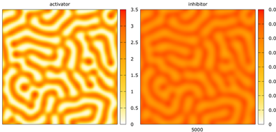
ActivatorInhibitor_2D.xml example model.
Check out ActivatorInhibitor_2D.xml to try yourself via:
- Morpheus Link or
- Morpheus GUI:
Examples→PDE→ActivatorInhibitor_2D.xmlor - Morpheus Model Repository.
In Space, it sets up a square lattice of $150 \times 150$ with periodic BoundaryConditions. The model itself is defined in the Global section where two diffusive Fields are created. The reaction step of the reaction-diffusion is specified in a System containing Constants and DiffEqns.
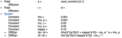
Global section of ActivatorInhibitor_2D.xml.
The plot above is created using the Gnuplotter plugin in the Analysis section, showing the concentrations of the two interacting species.
Field in Gnuplotter.
Global/Field/Diffusion to get finer patterns or no patterning at all.
CPM: Cell Sorting
This reproduces the first cellular Potts model that Graner and Glazier used to study cell sorting based on the differential adhesion hypothesis.
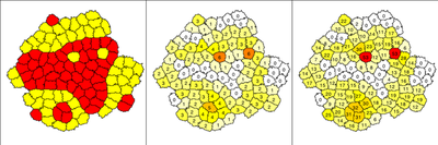
CellSorting_2D.xml example model. Cells are color-coded based on their CellType (left), number of neighbors of different type (center) and length of boundary to cells of other type (right).
Check out CellSorting_2D.xml to try yourself:
- Morpheus Link or
- Morpheus GUI:
Examples→CPM→CellSorting_2D.xmlor - Morpheus Model Repository.
Apart from specifying Space and Time, a number of CellTypes is specified. Each one has a VolumeConstraint to regulate the size of the cells. Remaining plugins are used to track the cell-cell boundary lengths.
In the CPM section, the Interaction energies are specified that control the ‘adhesion’ between cells of different cell types.
CPM-specific parameters such as the temperature of the MetropolisKinetics is also specified here. To define the spatial arrangement of cells in the lattice, in CellPopulations two Populations are described. These are initialized randomly in a circle using the InitCircle plugin.
A Gnuplotter is set up to visualize cells and a Logger is used to log and plot the boundary lengths.
CPM/Interaction.
Wrapping up
You probably have noticed some similarities and differences among these three models.
Clearly, each model defined the Space and Time of a simulation – even the non-spatial predator-prey model. These sections are indeed required. The Analysis section is not obligatory, yet all models use it since a simulation without output of any kind (plots or stats) is incomplete simulation.
Other sections such as CellTypes and CPM are optional and only appear when necessary. These are only used in the CPM example and do not appear in the ODE and PDE examples.
CellTypes but without using a cellular Potts model and therefore no optional CPM section (e.g. see ODE → LateralSignaling.xml).
The models above also show some useful ways to generate output from the simulations using the flexible Logger and Gnuplotter plugins.