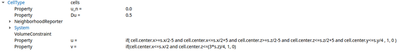
Convert to 3D
Now we finally arrive at the 3D model. As an example, we further develop the coupled PDE and CPM model with mechanical interaction.
Similar to the 1D to 2D case, it is straighforward to extend the dimensionality to 3D. We define the Lattice Size also in the z direction, i.e. 238,238,238 and set the structure (Lattice class) to cubic. The initial conditions now include the z dimension as well.
u and v.
u and v are not symmetric with respect to the dimensions anymore.
Check out barkley3d_coupling.xml to try yourself via:
- Morpheus-Link or
- Download:
barkley3d_coupling.xml
These initial conditions correspond to the following structure:
.](/media/course/from-pde-to-tissue/tutorial_3D_CPM-initial_huccfabc967d5c95b6beab0a2d32c7a34a_203344_730f3ab934c61e5e3990ce23172561b2.png)
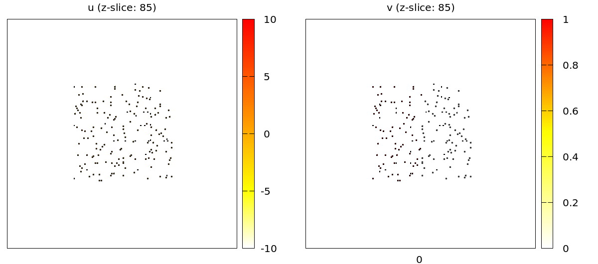
u (red) and v (blue). 3D visualization: ParaView.
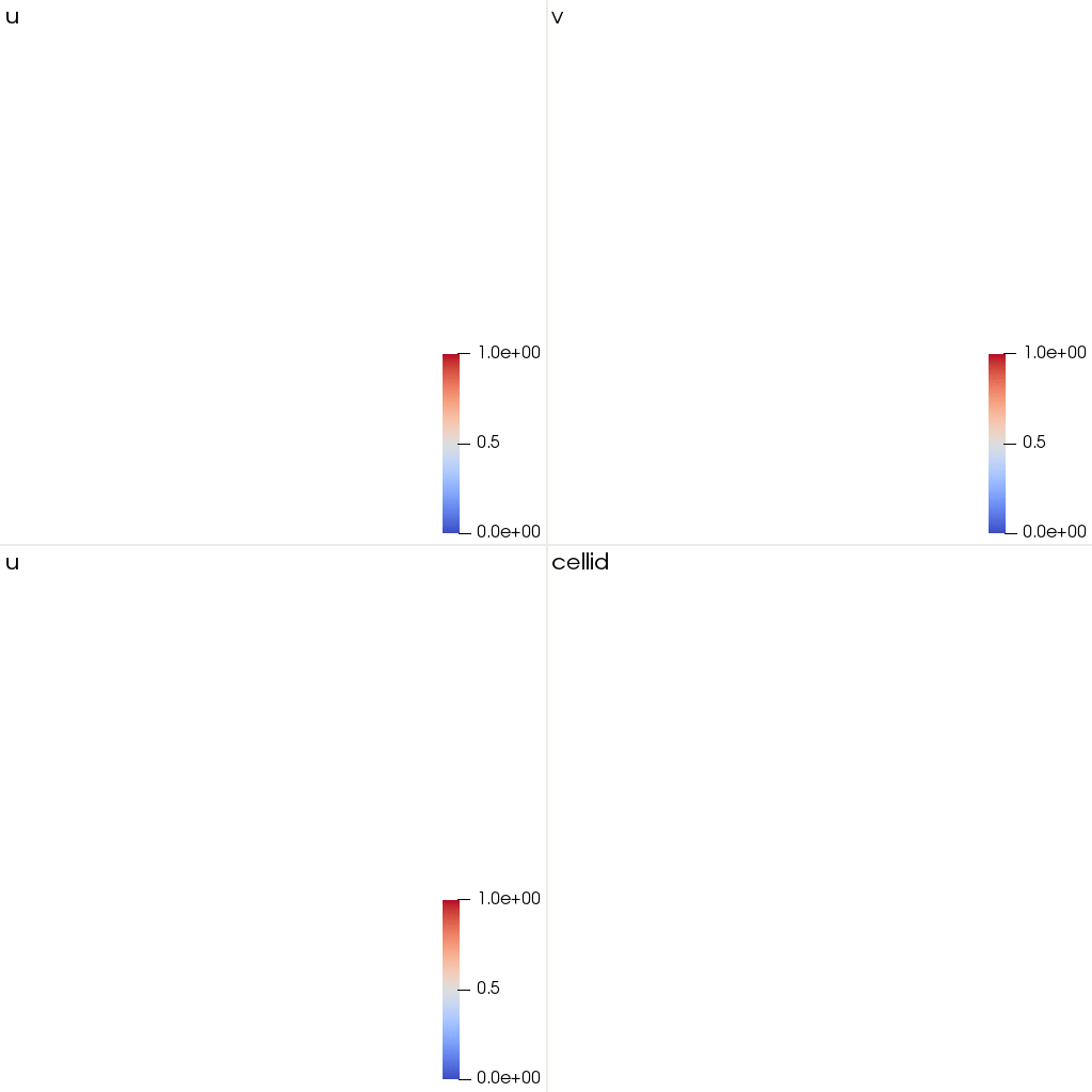
For visualization we can use Gnuplotter just like in the 2D case with the only difference that we have to indicate in the properties of the plot to show us just a single z slice.
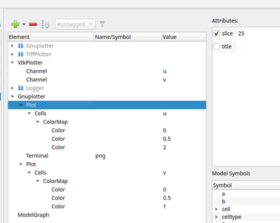
Gnuplotter in the Analysis section configured to plot z slice 25 of the 3D lattice.
For the full 3D data there are two plugins: the TiffPlotter and VtkPlotter. Here we use the VtkPlotter which plots one file for each time step that can then be visualized by the free software ParaView.