Convert to 2D
Converting the model from the previous chapter into a 2D model is trivial in Morpheus. In the Space section, you only need to change the Size of the Lattice to e.g. 20,20,0, and the Lattice class from linear to square.
Lattice Size=20,20,0 is pretty small, but for demonstration purposes we will use this system size in the following.
Spiral Waves
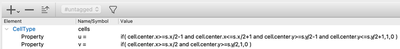
The most complicated part is to set up the initial conditions in order to get spiral waves. Here, we define u to be non-zero in a square in the middle of the lattice and v to be non-zero in the top-right quarter of the lattice. This suffices to obtain spirals. You can do this with an expression with CellTypes/CellType/Property or with CellPopulations/InitProperty similarly to the 1D model we have just discussed.
Without further changes, you will see a simulation with popagating spiral waves, in a discrete lattice of square cells.
Check out barkley2d_discrete.xml to try yourself via:
- Morpheus-Link or
- Download:
barkley2d_discrete.xml
Adding CPM Cells
To move away from these regular and static cells and add motility and cell mechanics, we will now include cellular Potts sampling to our model.
This is actually surprisingly easy. In our existing CellTypes section, we only need to add VolumeConstraint and a SurfaceConstraint that together make up the energy function for our cellular Potts model (CPM) to maintain a certain ratio between the size and the perimeters of the cells.
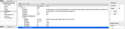
CellTypes section of the two-dimensional discrete model including the VolumeConstraint.
Check out barkley2d_cells.xml to try yourself via:
- Morpheus-Link or
- Download:
barkley2d_cells.xml
In addition, we need to specify some CPM-specific parameters in the CPM section of the model. In particular, we need to add a MonteCarloSampler and specify the temperature of the MetropolisKinetics which defines the amount of stochasticity in membrane fluctuations.
Another important parameter here is the MCSDuration. Typically, and by default, it is set to 1.0 to define one simulation time step as one Monte Carlo step (where on average every lattice point has been updated). Here, however, we want the simulation time to be determined by the dynamics of the Barkley model and scale the CPM model relative to this timescale. Here, we set the MCSDuration to 0.1 such that we simulate 10 CPM Monte Carlo steps for each simulation time step.
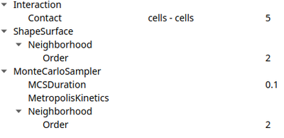
CPM section with MCSDuration=0.1.
Since our cells will now become larger than a single lattice site, we obviously need to increase the Size of the Lattice and change the initial configuration. We’ll use a InitRectangle to distribute our cell seeds over the lattice and InitVoronoi to render a Voronoi tessellation from these seeds.
Once set up, you will see a simulation like the one below. Note that the velocity and shape of the wave are not deterministic anymore because wave propagation is mediated by cell-cell contacts and these are governed by the stochastic cellular Potts model.
Coupling Signals to Biomechanics
In the simulation above, the CPM dynamics affect the wave propagation. However, the wave itself does not affect CPM. Now, we’ll add some juice and realize a mutual coupling between the intracellular dynamics and tissue mechanics.
Here, we will assume two types of coupling:
- We assume cells contract based on the concentration of
v. To implement this, we can use a mathematical expression instead of a value for the cell’s target areaVolumeConstraint/target: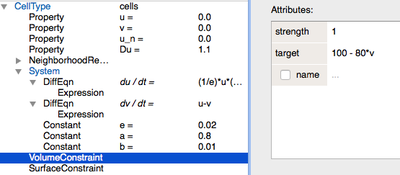
The VolumeConstraintdepends on the concentration ofv. - We assume that cells become more adherent to each other as a function of the concentration of
u. This can be modelled using theContactplugin underCPM/Interaction/Contact, optionally employing more specialised plugins such asHomophilicAdhesion. This modulates the cell-contact energy based on binding between two identical adhesives on adjacent cells, here represented byu.
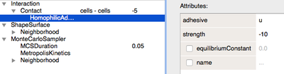
Interaction energies between cells depend on concentration of u.
Finally, to make the effect visually more dramatic, we do not simulate a confluent tissue, but only a fragment. We do this with the InitCellObjects initializer that let’s you arrange cells within geometric objects such as boxes or circles.
u and v concentrations are coupled to adhesion (CPM/Interaction/Contact energy) and VolumeConstraint/target.
As you can see, during the propagation of the wave, cells contract and become smaller due to the effect of the intracellular model variables on the cell mechanics. On the level of the tissue, we see cells moving back and forth in wavy patterns, which is most clearly visible at the tissue boundary.
Check out barkley2d_coupled.xml to try yourself via:
- Morpheus-Link or
- Download:
barkley2d_coupled.xml