1D PDE Barkley Model
Derived from the seminal Hodgkin-Huxley and FitzHugh-Nagumo models, the Barkley model is probably the simplest continuous model for excitable media. It replaces the cubic term in the FitzHugh-Nagumo model with a piece-wise linear term as a simplification that enables fast simulation.
The equations for the Barkley model are
$$ \begin{aligned} \frac{\partial u}{\partial t}&=\frac{1}{\epsilon}u(1-u) \cdot \left( u - \frac{v+b}{a} \right) + \nabla^2 u\\ \frac{\partial v}{\partial t}&=u-v \\ \end{aligned} $$
where the variable $u$ represents the fast dynamics and controls wave propagation and $v$ represents the slow dynamics controlling refractoriness. The parameter $\epsilon$ determines the time scale separation between the two dynamics, larger $a$ gives wider waves, increasing the ratio $\frac{b}{a}$ gives a larger excitability threshold.
Continuous Diffusion
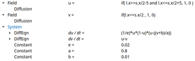
To simulate this model with Morpheus, we first define two Fields for u and v in the Global section. These define scalar fields, i.e. spatially resolved continuous variables over the whole lattice domain. Second, we define a System of differential equations (DiffEqn) for $\frac{\partial u}{\partial t}$ and $\frac{\partial v}{\partial t}$ and enter the reaction term of the equations above. Moreover, we specify the constants e, a and b. What is left is the diffusion rate for u, which is specified as 0.5 in Field/Diffusion.
Global section.
Check out barkley1d_cont.xml to try yourself via:
- Morpheus-Link or
- Download:
barkley1d_cont.xml
Once the core of the model is set up, we define a linear lattice with periodic BoundaryConditions in the Space section and the simulation duration with StopTime (here set to 100) in the Time section. To visualize the results, you can add a Logger and a Logger/Plot that records and plots the values of u and v over space and time.
As initial condition, we let u be non-zero in a patch (with the location l) in the middle of the lattice s:
if( l.x>=s.x/2-5 and l.x<=s.x/2+5, 1, 0 )
And v be non-zero in the left part:
if( l.x<=s.x/2 , 1, 0 )
This forces the wave to propagate to the right, as shown below.
Discrete Diffusion
Now, we want to reproduce this continuous spatial model with a discrete spatial model where each lattice site represents a biological cell. Later, we will expand this to 2D and add cellular dynamics using CPM.
In order to emphasize the discrete structure of the system, we first reduce the spatial resolution Space/Lattice/Size from 200 to 50 data points.
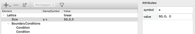
Lattice/Size.
Check out barkley1d_discrete.xml to try yourself via:
- Morpheus-Link or
- Download:
barkley1d_discrete.xml
Then, we take our System as defined in Global before, but move it to a CellType in the CellTypes section. So instead of a scalar field, we now want every cell to compute the reaction part for itself. That is, we convert the PDE to an ODE system.
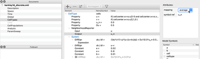
CellTypes section of the discrete model.
System from Global to CellTypes.
Furthermore, as you can see from the figure above, we need to adjust three more things in the CellTypes section:
-
To spatially couple the ODEs, we use a
NeighborhoodReporterthat looks at the value ofuin the neighboring cells and returns theaverageof these values, which is assigned to the newPropertyu_n. -
In the reaction term of $\frac{\partial u}{\partial t}$, we now add
Du*(0.5*u_n - 0.5*u)that defines the discretized version of diffusion, which can be interpreted as an undirected cell-to-cell transport term. The propertyDuis then set to the same value (0.5) as the diffusion rate in the continuous model. -
To specify the initial values of
uandvwe now put our mathematical expressions, instead of inGlobal/Fieldas described above for the continuous model, in the respectivePropertyinCellTypes/CellType.
To specify these initial values, you can alternatively use the InitProperty plugin in the CellPopulations section.
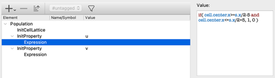
CellPopulations/InitProperty.
However, since we only need one cell population, we can simply set our initial values directly on the CellType level.
Besides the initial values, the initial state of the system also includes the spatial distribution of the cells. Therefore, in the section CellPopulations we finally add the plugin InitCellLattice which initializes a population of cells in which each lattice site is filled with exactly one cell.
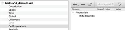
InitCellLattice.
To visualize the behavior of this system, you can use a Gnuplotter and color-code the cells using the u and v properties and see something like this: