Anisotropy of CPM shape boundary estimation

Last updated on Wed, 04 Oct 2023 4 min read

Neighborhood choices

Neighborhood choices in CPM simulations are not only fundamentally coupled to their parametrization, but also cause profound implications on cell shape and cell dynamics anisotropy. While in part 1 we addressed the decoupling of neighborhood choices and parametrization, here we evaluate interaction neighborhoods wrt. the cell shape implications.

Shape anisotropy

The CPM dynamics is defined by an optimization algorithm minimizing the Hamiltonian energy of the system. Thus, energy anisotropies of the Hamiltonian potential wrt. the underlying lattice render certain cell shape alignments favourable, leading to so-called lattice-artifact.

Since both, the perimeter constraint and the contact energy depend on the estimate of perimeter / surface lengths, we study the impact of a shape’s orientation wrt. the lattice axes and the neighborhood size on the accuracy of perimeter / surface length estimation.

Square lattice

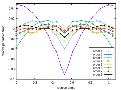
A square shape of sufficient extend can serve as a test object on the square lattice to quantify the lattice-artifact of perimeter length estimation. If rotated by an angle φ (see CPM configuration below), all of it’s sides are tilted by this same angle wrt. the lattice axes.

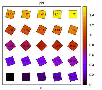
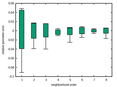
We know the expected perimeter (in continuous space) given the discretized square’s size and below compare it to the estimated perimeter using different neighborhood kernels of specified order (color-coded) and the correction factor ξ as defined in part 1.

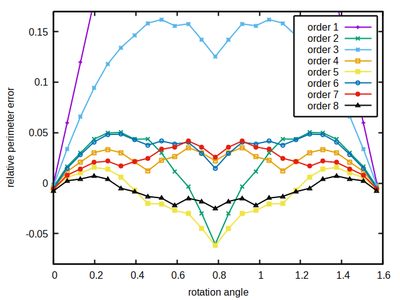
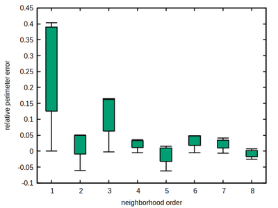
Angle-dependent relative error of perimeter length estimation (revealing anisotropy) for different neighborhood orders (color-coded) measured for square shapes as above

Numerical estimation error for each neighborhood order

As a rule of thumb, the larger the better holds for the neighborhood order. However neighborhood order 4 turns out to be a sweet spot for the square lattice, combining a moderate size with a comparably low and flat accuracy error profile, thus minimizing the occurrence of local energy minima that may provoke spatial shape artifacts (locking-in of cell edges at preferred angles with over- or under-estimation of edge length depending on the volume vs. perimeter constraints).

Hexagonal lattice

A hexagon shape of sufficient extend can serve as a test object to estimate the accuracy of perimeter length estimation in a hexagonal lattice. If rotated by an angle φ, all of it’s sides are tilted by this same angle wrt. the 3 lattice symmetry axes, see below.

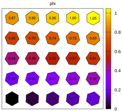
We know the expected perimeter from the discretized hexagon’s size and then measure the perimeter using a neighborhood kernel of specified size (color-coded) and the correction factor ξ as described in part 1.

Angular anisotropy of perimeter estimation error for different neighborhood orders (color-coded) of hexagon shapes

As a rule of thumb, the larger the better also holds here. However, again neighborhood order 4 turns out to be a sweet spot for the hexagonal lattice, combining a moderate size with a comparably low and flat accuracy error profile, thus minimizing the occurrence of local energy minima that may provoke spatial shape artifacts.

Cubic lattice

Cubes of sufficient extend can serve as a test object to estimate the accuracy of surface size estimation in a cubic lattice. If rotated by an angle φ in x,y-plane and by elevation ϑ=φ, all of it’s sides are tilted by the same angle wrt. the 3 lattice axes.

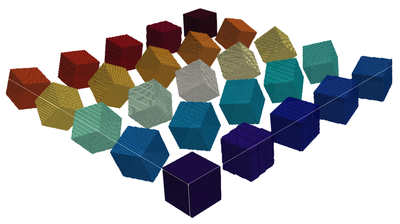
We know the expected surface from the discretized cube’s size and then measure the surface using a neighborhood kernel of specified size (color-coded) and the correction factor ξ as defined in part 1.

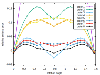
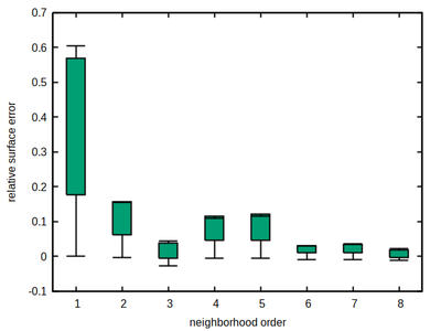
Angular anisotropy of surface estimation error of tilted cubes for neighborhood orders (color-coded)

The rule of thumb, the larger the better also holds here. Remarkably, a significant improvement occurs at order 6, rendering this order as a sweet spot for the cubic lattice, combining a moderate size with a comparably low and flat accuracy error profile, thus minimizing the occurrence of local energy minima that may provoke spatial shape artifacts.

Summary

All 3 lattices - hexagonal, square and cubic - provide a sweet spot in the choice of neighborhood order. This respective neighborhood should be preferred for simulations that are sensitive to cell shapes and spatial cell dynamics. The lowest anisotropy among these optimal lattice neighborhoods, measured by the variance of the relative estimation error, is reached by the hexagonal lattice 4th order neighborhood with a variance of 2.7e-5, while the 6th order on cubic lattice reaches 9.7e-5, and the 4th order on square lattice reaches 1.4e-4 only.

Within Morpheus, this preferred neighborhood is selected as a default – namely by the optimal neighborhood choice.

As an open question remains, whether the correction factors ξ for scaling a neigbhborhood kernel to continuous space boundary lengths (see also Magno et al.), is best estimated based on the whole angular estimate profile - as we did for the hexagonal case in part 1, or rather from the axis parallel boundaries only - as done for the square and cubic case by Magno et al..

References

Magno, R., Grieneisen, V.A. & Marée, A.F. The biophysical nature of cells: potential cell behaviours revealed by analytical and computational studies of cell surface mechanics. BMC Biophys 8, 8 (2015).